External MPC Unit Discussion Paper No. 36 Did output gap measurement improve over time? Adrian Chiu and Tomasz Wieladek July 2012
This document is written by the External MPC Unit of the Bank of England
External MPC Unit Discussion Paper No. 36 Did output gap measurement improve over time? Adrian Chiu(1) and Tomasz Wieladek(2) Abstract We study whether the accuracy of real-time estimates of the output gap produced by the OECD has improved over time by examining a panel dataset on real-time output gap revisions for 15 countries from 1991 Q1 — 2005 Q4. We use a simple panel data regression and a state space model, with common and country-specific factors, to assess whether the mean of the absolute value of output gap revisions has changed. We also apply a Mincer-Zarnowitz regression to determine whether the composition of measurement errors has shifted. Surprisingly, we do not find evidence that the size of output gap revisions has decreased over time; on the contrary, they seem to have increased. But the fraction of measurement errors due to omitted contemporaneous information has declined. This suggests that while the OECD’s accuracy in output gap measurement has failed to improve, its estimates are becoming less noisy. Keywords: Output gap, real-time data, dynamic common factor model. JEL classification: E01, E32.
(1) Bank of England. Email:
[email protected] (2) Bank of England. Email:
[email protected] These Discussion Papers report on research carried out by, or under supervision of the External Members of the Monetary Policy Committee and their dedicated economic staff. Papers are made available as soon as practicable in order to share research and stimulate further discussion of key policy issues. However, the views expressed in this paper are those of the authors, and not necessarily those of the Bank of England or the Monetary Policy Committee. Information on the External MPC Unit Discussion Papers can be found at www.bankofengland.co.uk/publications/Pages/externalmpcpapers/default.aspx External MPC Unit, Bank of England, Threadneedle Street, London, EC2R 8AH © Bank of England 2012 ISSN 1748-6203 (on-line)
1. Introduction As is well known, real-time estimates of the output gap are often subject to considerable revision over time.1 This unreliability of real-time output gap measures has been widely documented for the US (Orphanides and Van Norden, 2002), the UK (Nelson and Nikolov, 2003), Canada (Coyen and Van Norden, 2005), Norway (Bernhardsen, Eitrheim, Jore and Roisland, 2004 ), as well as several other OECD countries (Tosetto, 2008). This is a serious problem for monetary policy makers; for example, as Orphanides (2001) documents, an output gap measurement mistake led the Federal Reserve to pursue policies that eventually led to the Great Inflation of the 1970s. Similarly, Nelson and Nikolov (2003) document that output gap measurement mistakes led to interest rate settings that deviated about 500 basis points from what would have been consistent with the actual output gap during the ‘Lawson boom’ in the UK.2 At the same time, there are reasons to believe that the accuracy of real-time output gap estimates may have improved over time. In particular, a number of research papers raised awareness of the scope and implications of these measurement problems in the 1990s. This may have led to an increase in resources to solve them. Modern computing and communication technology also allowed analysts to incorporate a much greater amount of contemporaneous information into their initial output gap estimates, probably helping them to minimise measurement errors associated with data noise. Finally, several OECD countries introduced various business surveys reporting on spare capacity in various parts of the economy; these are likely to improve initial output gap estimates. In other words, as a result of these methodological changes, the size of past output gap mistakes may not be a good guide to the present.
1 Orphanides and Van Norden (2002) document three main reasons for output gap measurement errors. First and most obviously, real GDP data is often revised – sometimes substantially – after the initial estimates are published. Second, there is considerable uncertainty in the level of potential output at any point in time. Finally, researchers might also change their methodology for estimating potential GDP, or their assumptions within chosen methods, over time 2 The Lawson boom was an unsustainable period of fast real GDP growth and rising prices in the UK in the late 1980s, as a result of low interest rates. This time period was named after Nigel Lawson, the UK’s Chancellor of the Exchequer at the time.
Discussion Paper No. 36 July 2012
2
To assess whether this is the case, we examine changes in the absolute values of output gap revisions (hereafter ‘absolute output gap revisions’) in a panel data set of 15 OECD countries from 1991Q1 to 2005Q4. Initially, we use a simple panel data model to test whether the mean of absolute output gap revisions has changed over time; we do this by estimating the model over two different time subsamples and a rolling window of 16 quarters. We then use a more flexible dynamic common factor model, with both a common factor and country-specific factors, to verify these results. Finally, we examine whether the decomposition of output gap revisions between ‘news’ and ‘noise’ has also changed over time3. We argue that improvement in information processing associated with modern communication and computing technology should probably reduce the size of measurement errors due to delayed inclusion of information available at the time. To test this hypothesis, we estimate a Mincer-Zarnowitz (1969) forecast efficiency regression, as before, across two different sub-samples and on a rolling window of 16 quarters. Our results fail to find evidence of a decline in the size of absolute output gap revisions over time; on the contrary, these revisions seem to have increased. But we do find that the fraction of output gap revisions due to the delayed inclusion of contemporaneous information has indeed declined. This suggests that, while statisticians did become better at processing contemporaneous information into real-time estimates of the output gap, these estimates did not improve in accuracy, perhaps due to the difficulty of disentangling the trend and the cycle. The rest of this paper is structured as follows. Section 2 describes the data and section 3 the empirical methodology. Section 4 presents the results and section 5 concludes.
3 Revisions can occur either as a result of delayed inclusion of information available at the time initial output gap estimates were made (the ‘noise’ view), or new information which was not available at the time (the ‘news’ view).
Discussion Paper No. 36 July 2012
3
2. Data Our data are taken from the OECD’s real-time output gap database, first published in August 2008.4 This database contains real-time output gap estimates for 15 OECD countries for the period from 1991 Q1 onwards. We treat the output gap figures published in the 2010 Q4 OECD Economic Outlook as our ‘final’ vintage of output gap data. Output gap revisions are constructed by subtracting the real-time estimate of the output gap (hereafter, ‘real-time vintage’) at each point in time from its 2010Q Q4 estimate (‘final vintage’). We judge that real-time vintage output gap estimates towards the end of our sample could still be significantly revised in the future, which may introduce bias in our estimates. To mitigate this problem we drop any observation past 2005Q4. The OECD defines the output gap as actual real GDP minus potential real GDP, as a percentage of potential real GDP (Tosetto, 2008). Potential real GDP is defined as the level of output that an economy can produce at a constant rate of inflation. However, unlike actual GDP, it cannot be directly observed from economic data. The OECD therefore indirectly infers the output gap from economic data using a ‘production function’ approach, rather than relying on mechanical time-series filters to measure potential output. This could mean that output gap measurements include the judgement of OECD country analysts, similar to the process followed in many central banks today.5 Another advantage of using OECD data for this investigation is that the similarity in methodology makes output gap estimates comparable across countries.
4 5
http://www.oecd.org/document/1/0,3343,en_2649_33715_41054465_1_1_1_1,00.html For details on this method, see Giorno, Richardson and Roseveare and Van Den Noord (1995).
Discussion Paper No. 36 July 2012
4
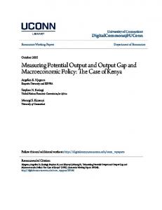
Figure 1: Distribution of output gap revisions 160
Mean = 0.36 Std. Dev. = 1.25 Skewness = ‐0.65 Kurtosis = 7.47
140 120 100 80 60 40 20 0
Figure 1 shows the distribution of output gap revisions in the OECD database for all 15 countries, for the period 1991 Q1 to 2005 Q4. 64% of all revisions have a positive value, suggesting that a positive revision is more likely than a negative one. It is centred around a mean of 0.36, which is roughly 43% of the average size of real-time output gap estimates in our sample.
3. Methodology In this study we aim to assess whether the accuracy of output gap estimates made in real time has improved over time. We measure accuracy as the absolute value of output gap revisions, since we are interested in the size rather than the sign of any error. First we test whether the size of the mean of absolute output gap revisions has changed between the 1990s and 2000s with a simple panel data model. To provide greater detail on how the mean of absolute value output gap revisions has changed over time, we re-estimate the same model over a rolling window of 16 quarters. We also estimate rolling regression coefficients for the same model to assess how the mean of the absolute output gap revisions has changed over time. We then use a more sophisticated dynamic common
Discussion Paper No. 36 July 2012
5
factor model, with both a common factor and individual country-specific factors, to verify these results. In the final section, we examine whether the composition of revisions has changed over time with a Mincer-Zarnowitz regression approach. In particular, one would have expected that with the introduction of modern communication and computing technology, and the associated improvements in information processing, the fraction of measurement error due to the delayed inclusion of contemporaneous information should have declined over time. As before, we first estimate the Mincer-Zarnowitz regression model over two subsamples and then on a rolling window of 16 quarters. 3.1 Panel data model We begin to explore our data set with a simple panel data model. We start by estimating the following regression equation6: ,
where
,
,
,
,
is the absolute output gap revision,
(1) a country-specific fixed effect and
dummy variable, which takes the value of one for any time period after 2000 Q1.
,
a
is
therefore the coefficient of the greatest interest to us, as its sign and the degree of statistical significance will be informative of whether the size of revisions did change over time. The choice of this particular break point may be seen as arbitrary. To address this, we estimate equation (1a) below for overlapping rolling window of 16 quarters. ,
,
,
(1a)
We then plot the resulting mean of absolute output gap revisions and its 95th confidence band to assess how it has evolved over time.
6
There are alternative approaches to testing for structural breaks; for example, see Zivo t and Andrews (1992).
Discussion Paper No. 36 July 2012
6
3.2 Dynamic Common Factor model Model (1a) might seem restrictive once it is considered that there are at least two different ways in which the mean of absolute output gap revisions can change over time. Some improvements in technology, in particular in information processing due the availability of faster computers, would probably lead to changes in revisions which are common to all the 15 OECD countries in our sample. At the same time, the availability of business surveys of spare capacity could lead to country-specific changes in output gap revisions. Similarly, errors in judgement about the cycle and the trend could occur either at the global or country-specific level. The common and country-specific component could therefore conceivably be moving in opposite directions. In this case, the simple panel data model presented in 3.1 would suggest the absence of a change when it is actually present. To verify the results from the simple panel data model, we therefore use a Bayesian dynamic common factor model with one common factor and individual country-specific factors. In previous applications, such methods have been employed to study and identify the international business cycle from domestic investment, consumption and output data across a range of countries, and to quantify the contribution of the world ‘factor’ (representing the world business cycle) to their variation. Applied to the question at hand, the common factor may reflect changes in absolute output gap revisions which are in common to all of the countries. Similarly, the country-specific components will reveal whether the size of absolute revisions has changed at the country level. We implement the following model: ,
,
,
,
,
,
,
,
~
0,
(2)
~
0,
(3)
~
0,
(4)
Discussion Paper No. 36 July 2012
7
,
where
,
,
0,
,
0,
,
(5)
is the absolute output gap revision in country i at time t,
specific factor that evolves according to a random walk, drives time series in all of the countries and
variation and
is a country-
is a common factor which
is the country-specific factor loading is the covariance matrix of the
relating the factor to the individual country time series. idiosyncratic component,
,
the covariance matrix governing the shocks to time-
the variance of the common factor. Both
,
and
,
are country-specific
and would, in any conventional state space model, be observationally equivalent. To ensure that we can separate the two, we model
,
as a time-varying mean, which only
evolves slowly over time. This is achieved via a fairly tight prior on
, the matrix
governing the size of time-varying shocks, to embody our belief that changes in output gap measurement technology only occur slowly over time.7 For simplicity of notation we will refer to this model in the following state space form for the rest of the paper:
,
~
0,
(6) ~
where
;
,
…
,
and
; 1… 1
0,
(7)
where k is the number of countries.
The matrix H contains the corresponding factor-loadings as well as an identity matrix to account for the fact that the a square matrix with matrix with
,
and the
’s enter the measurement equation in levels directly. G is ’s on its diagonal.
,
…
,
and
is a square
’s on the diagonal
7 This specification follows the approach presented in Cogley and Sargent (2001) and Del Negro and Otrok (2008) who also model time variation as smoothly changing coefficients across periods to capture permanent structural change.
Discussion Paper No. 36 July 2012
8
3.2.1 Dynamic Common Factor model – Identification From a purely statistical point of view, the above model is subject to two distinct identification problems: neither the scales nor the signs of the factor and the factor loadings are identified. Like most dynamic common factor models, our model is subject to the problem that the relative scale of the model is indeterminate. One can multiply the vector of factor loadings, Γ , by a constant d for all i, which gives by d, which yields to the scale of the model
. The scale of the model
. We can also divide the factor is thus observationally equivalent
. In order to solve this problem, we take the approach that is
widely applied elsewhere and set N, the variance matrix of the error term of the factor to 1. In addition, the model is subject to the rotational indeterminacy problem (Harvey (1993)). For any k x k orthogonal matrix F there exists an equivalent specification such that the rotations
and
produce the same distribution for
as in the
original model. This implies that the signs of the factor loadings and the common factor are not separately identified. This can be easily seen when setting F=-1, as in this case and
are observationally equivalent. In order to solve this problem we follow
Del Negro and Otrok (2008) and impose one of the factor loadings to be positive, as this permits the identification of the sign of the factor and thus the rest of the model. From an economic point of view, the common factor
is likely to capture
unobserved factors that are associated with improvements in methodology that all countries experienced simultaneously. This could be, for instance, an improvement in information processing as a result of better computer technology. The country-specific factors are likely to capture changes in country-specific measurement, such as the availability of various spare capacity business surveys.
Discussion Paper No. 36 July 2012
9
3.2.2 Dynamic Common Factor model - Implementation Dynamic factor models can be estimated with maximum likelihood methods (Gregory, Head and Raynauld (1997)). Nevertheless, with a large number of series in the cross-section, the resulting likelihood functions may have odd shapes (Bernanke, Boivin and Eliasz (2005)). To address this problem, Kose, Otrok, and Whiteman (2003) use the methods introduced in Carter and Kohn (1994) to develop a Bayesian Kalman filter procedure, which permits them to estimate large dynamic common factor models easily. The model is estimated with a Bayesian technique, Gibbs sampling. Typically, researchers ‘de-mean’ the data by subtracting them from their own averages, and standardize the variances to unity prior to estimating a dynamic common factor model. We follow previous work in standardizing the variances to unity, since this will prevent the most volatile series in the data from dominating the evolution of the common factor. But since we plan to model the mean of each series explicitly via the country-specific factors, we do not ‘de-mean’ the data. One crucial decision is the prior on
, the variance-covariance matrix of the
disturbance term of each country-specific factor, which governs the amount of timevariation. We follow the approach set out in Cogley and Sargent (2001) and set the prior on
proportional to the variance-covariance matrix of the country-specific time series.
We thus set
where
is a proportionality constant. Intuitively,
can be
described as the uncertainty surrounding the time-varying means. Given that we standardised the data to have a standard deviation of 1,
1. Setting
=.035 for
instance would impose a prior that time variation cannot explain more than 3.5% of the uncertainty around . Cogley and Sargent (2001) suggest that this value for
is
conservative, but realistic to explain permanent structural change in quarterly data. We follow their suggestion, but a higher (.1) or lower (.01) value of
does not change our
results qualitatively. Please see appendix A for greater details about the estimation procedure.
Discussion Paper No. 36 July 2012
10
Testing for convergence We replicate the above algorithm 100,000 times with Gibbs sampling and discard the first 50,000 replications as burn-in, keeping only every 10th draw in order to reduce auto-correlation among the draws. We then obtain the parameter estimates of the posterior distribution from the last 5,000 replications by taking the median and constructing 95% quantiles around it. We follow previous work and try various length of the iterative process. The results do not change, whether we replicate the model 100,000 times and retain 10,000 draws or replicate it 10,000 times and retain the final 1,000 draws for inference. Two possible test for convergence in our case are the two-sided KolmogorovSmirnov and Cramer-von-Mises test. These tests permit the statistical assessment of whether the underlying distribution behind two random samples is the same. We split the retained 5,000 draws in two samples and test whether they differ. Since we could never reject the null hypothesis that both samples come from the same distribution, we conclude that our procedure always seems to converge. 3.3 Mincer-Zarnowitz regression model Apart from the size, the composition of output gap measurement errors could have changed over time as well. Previous work by Boschen and Grossman (1982), Mankiw, Runkle and Shapiro (1984), Mankiw and Shapiro (1986), Maravall and Pierce (1986), Mork (1987, 1990), Patterson and Heravi (1992), Croushore and Stark (2001, 2003), Faust, Rogers and Wright (2005), Swanson and Van Dijk (2006), and Aruoba (2008) argues that revisions to real-time output gap estimates invariably fall into two categories, labelled ‘news’ and ‘noise’. We follow this classification here. Under the ‘noise’ category, measurement errors are uncorrelated with the true values. They pollute the preliminary output gap data and would need to be filtered out in order for the preliminary number to become an optimal estimate. If revisions are mostly due to ‘noise’, real-time output gap measurement errors – thus revisions to output gap estimates – might be reduced by
Discussion Paper No. 36 July 2012
11
increasing the resources dedicated to incorporating omitted contemporaneous information. On the other hand, under the ‘news’ category, revisions are the result of the arrival of new information about the state of the economy, which is not available at the time of measurement. In this case, the estimate can only be improved after the inclusion of such additional information. To measure the relative importance of ‘noise’ and ‘news’, we follow Faust, Rogers and Wright (2005) and express the preliminary data error term
, i.e.
as the sum of final data
and an
. Under the ‘news’ view, the real-time output gap reflects
all information available at the time of the data release. In this case information available after the release, implying that
and
will only reflect
are uncorrelated. On the
other hand, if all of the revision were due to subsequent inclusion of information available at the time of release,
would be uncorrelated with
. In intermediate case
will, of course, be correlated with both. As in Faust et al, we run what is essentially a forecast efficiency test, sometimes known as the Mincer-Zarnowitz (1969) test, to distinguish between these two views. If news explain all of the measurement error, then the revision, i.e. the difference between
and
, should be uncorrelated with any
information available at time t. But if revisions at least in part reflect noise, would be correlated. In particular,
and
would predict the revisions. Formally, the
regression is: ,
where
is a fixed effect and
(8)
,
,
. The Mincer-Zarnowitz (1969) procedure is
in essence an F-test of the null-hypothesis that
0, which would imply that
output gap revisions are unpredictable. To assess whether statistical authorities have improved upon their ability to incorporate contemporaneous information into preliminary data releases, we estimate this regression for the 1990s and 2000s separately. As before, we also report rolling regression estimates obtained with a 16 quarter window for verification.
Discussion Paper No. 36 July 2012
12
4. Results 4.1 Panel-data model Estimates of equation (1) are presented in Table 1. Our interest is to assess whether there is a statistically significant difference in the mean of the absolute output gap revisions between the 1990s and 2000s. According to the results in Table 1, we can reject the null-hypothesis that
0. Indeed, the fact that
is highly statistically
significant and positive suggests that the mean absolute output gap revision has become larger over time. Table 1 Panel data model Constant
0.86
(std. error)
(0.03) 0.18
(std. error)
(0.05) 2
Adjusted R
0.30
Figure 2 shows the estimates of the mean of the output gap revisions obtained with a rolling panel fixed effects regression, together with its 95% confidence band. The first observation reflects the estimate for the time between 1991Q1 and 1994Q4. As one can clearly see, the mean of absolute output gap errors seems to have increased towards the end of our sample, which is consistent with the results presented in Table 1.
Discussion Paper No. 36 July 2012
13
Figure 2: Five-year moving average revision and its 95% confidence band 1.3 Mean
1.2
Upper 95% confidence band Lower 95% confidence band
1.1 1.0 0.9 0.8 0.7 0.6
1995
1996
1997
1998
1999
2000
2001
2002
2003
2004
2005
4.2 Dynamic common factor model We present all of the results from the dynamic common factor model below. Figure 3 depicts the common factor together with 95% confidence bands.8 The common factor does not seem to move much during the 1990s, but increases in the 2000s. Although this result is not statistically significant, interestingly, the dynamic common factor evolves in a way similar to the estimate from the rolling panel data model obtained over a window of 16 quarters. It also confirms the result that the mean of the absolute output gap error seems to have increased over time.
8
Note that if the distribution of the common factor were to be normal, then these would be equivalent to standard 95th percentile confidence bands.
Discussion Paper No. 36 July 2012
14
Figure 3: Dynamic Common Factor 7
6
5 % C o v e ra g e B a n d M e d ia n 9 5 % C o v e ra g e B a n d
5
4
3
2
1
0 1991Q 1
1994Q 4
1998Q 4
2002Q 4
2005Q 4
Figure 4 shows the country-specific factors together with the associated 95th confidence intervals. There does not seem to be a pattern of declining mean absolute output gap revisions, other than for Finland and Australia. But even in these cases this pattern is not statistically significant. In some countries, like the US, Italy and Ireland, on the other hand, mean absolute output gap revisions seem to increase over time. In most other countries, there does not appear to be a clear trend towards an increase or decrease in the mean absolute output gap revision over time.
Discussion Paper No. 36 July 2012
15
Figure 4: Time-varying mean coefficients C anada
A us tralia 2
2
1
1
0
0
-1
-1
-2 1991 Q 1
19 98Q 4
2005Q 4
-2 1991Q 1
1998Q 4
G erm any
F inland
2
2
1
1
0
0
-1
-1
-2 1991 Q 1
19 98Q 4
2005Q 4
-2 1991Q 1
1998Q 4
F ranc e 1
2
0.5
1
0
0
-0.5
-1
-1 19 98Q 4
2005Q 4
Ic eland
3
-2 1991 Q 1
2 005Q 4
2005Q 4
-1.5 1991Q 1
1998Q 4
2005Q 4
5% P os terior C ov erage B and M e dian 95% P os te rior C ov erage B and
Discussion Paper No. 36 July 2012
16
Figure 4: Time-varying mean coefficients - continued Ireland
Italy
2
1.5
1
1 0.5
0
0 -1 -2 1991Q 1
-0.5 1998Q 4
2005Q 4
-1 1991Q 1
J apan
1998Q 4
2005Q 4
N etherlands
1
1.5
0.5
1 0.5
0
0 -0.5 -0.5 -1 1991Q 1
1998Q 4
2005Q 4
-1 1991Q 1
N orw ay 2
0.5
1
0
0
-0.5
-1
1998Q 4
2005Q 4
N ew Z ealand
1
-1 1991Q 1
1998Q 4
2005Q 4
-2 1991Q 1
1998Q 4
2005Q 4
5% P os terior C ov erage B and M edian 95% P os terior C ov erage B and
Discussion Paper No. 36 July 2012
17
Figure 4: Time-varying mean coefficients - continued S w e den
UK
1.5
1 .5
1
1
0.5
0 .5
0
0
-0.5
-0 .5
-1 1991 Q 1
199 8Q 4
2005 Q 4
-1 1 991Q 1
1998 Q 4
2 005Q 4
US 1.5 1 5% P os terior C ov e rag e B a nd M ed ian 95 % P os te rior C ov era ge B and
0.5 0 -0.5 -1 -1.5 1991 Q 1
199 8Q 4
2005 Q 4
4.3 Mincer-Zarnowitz Regressions Table 2 presents estimates of equation (9) for two different time periods. For the sample as whole, an F test rejects the null-hypothesis that
0, suggesting that
revisions are predictable.
Discussion Paper No. 36 July 2012
18
Table 2 1991Q – 2005Q4
1991Q1 – 1999Q4
2000Q1 – 2005Q4
Constant
0.13
0.17
0.27
(std. error)
(0.03)
(0.03)
(0.06)
Prelim
-0.27
-0.20
-0.47
(std. error)
(0.01)
(0.01)
(0.04)
F
40.61
57.48
20.14
(0.00)
(0.00)
(0.00)
0.40
0.61
0.44
(p-value) 2
Adjusted R
For the sample up to 2000Q1, the adjusted
of .61 suggests that roughly 60% of the
revision can be explained by omitted information available at the time the preliminary estimate, with the rest due to information only available later. Repeating the same exercise for the sample after 2000Q1 suggests that only 44% of the revision can be explained by omitted contemporaneous information at the time of the preliminary output gap release. One may thus conclude that the fraction of output gap revisions as a result of noise appears to have fallen over time. As before, we also re-estimate this regression over a rolling window of five years to assess how the split between news and noise has changed over time. The results are shown in Figure 5; the 1995 value, for example, would correspond to the adjusted
and F-statistic of
the Mincer-Zarnowitz regression for the period 1991Q1 to 1994Q4. Although the F-Statistic has fallen over time, the null-hypothesis that
0 is still rejected at the 5% level at
each point in time, suggesting that revisions are always predictable. The
falls from about
.7 to .4 at the end of the sample, confirming the earlier result that the proportion of noise in the preliminary GDP estimates has consistently fallen over time.
Discussion Paper No. 36 July 2012
19
Figure 5: Adjusted R-square and F-statistics for five-year rolling MincerZarnowitz regressions 70
0.8
60
0.7 0.6
50
0.5 40 0.4 30 0.3
Adj. R-square (RHS) 20
F-stat (LHS)
0.2
10
0.1 0.0
0 1995
1996
1997
1998
1999
2000
2001
2002
2003
2004
2005
5. Conclusion A large body of research has shown that real-time estimates of the output gap tend to be unreliable. Greater awareness of this problem and increases in the resources devoted to a possible solution may have contributed to greater accuracy of real-time estimates of the output gap. Similarly, advances in our capability to process ever greater amounts of information in real time, as a result of technological innovation, should have led to a reduction of data noise as a result of omitted contemporaneous information. In this paper, we examine if either the size or composition of revisions in the output gap estimates produced by the OECD have changed over time. We exploit an OECD database on output gap revisions in 15 countries from 1991Q1 to 2005Q4 to answer this question. We use both a simple panel-data model and a more sophisticated dynamic common factor model with country specific factors to examine whether the mean of absolute output gap revisions has changed over time. Furthermore, we use the Mincer-Zarnowitz regression approach to assess if the composition of revisions has changed. We find evidence that the absolute level of output gap revisions have increased over time. We also find that the fraction of output gap revisions due to omitted contemporaneous information (data noise) has declined. This
Discussion Paper No. 36 July 2012
20
suggests that while economists did become better at real-time data processing, this failed to translate into a reduction in the absolute size of output gap revisions, possibly due to the difficulty in separating the trend from the cycle in economic data. The size of the output gaps in OECD countries is frequently cited as one of the main reasons behind the loose monetary policy implemented following the global financial crisis of 2008. Understanding how well this concept is measured and whether real-time estimation has improved over time is therefore an important policy question. In this paper we found that the composition, but not the size, of output gap revisions has changed over time. Future research should aim to shed light on why this is the case and what can be done to reduce the size of measurement errors of this important variable.
Discussion Paper No. 36 July 2012
21
Appendix A Dynamic Common Factor model - Estimation Estimation with Gibbs sampling permits us to break the estimation down into several steps, which reduces the difficulty of implementation drastically. For instance, if the unobserved dynamic common factor in equation (4) would be known, then the estimation of the factor loadings,
, would involve a simple OLS regression. Similarly, if
the factor loadings are known, then the estimation of the unobserved factors only involves the application of Kalman filter to the state space form of the model in equation (6). Finally, given knowledge of the dynamic common factor, the estimation of the autoregressive parameter in equation (4) can be performed through a simple regression of the lagged factor on itself. For this purpose we employ a Gibbs sampling algorithm that approximates the posterior distribution and describe each step of the algorithm below.
Step 1 - Estimation of the factor-loadings on all other parameters Conditional on a draw of matrix
, we draw the factor loadings
and the covariance
. With knowledge of all the other parameters we can estimate each factor
loading
via OLS regressions separately. The posterior densities which we use to achieve
this are: ,
where
,
,
,
and ∆
,
, ,
~N
,
,∆
(9)
.
Discussion Paper No. 36 July 2012
22
Step 2 - Estimation of the dynamic common factor and the time-varying means We can now obtain an estimate of filter.9 We assume
with the Bayesian variant of the Kalman
to be latent and unobservable. We draw
conditional on all
other parameters from
, H, , , H, ,
~N ~N
, , ,H,
,H,
,P
,P
,
(10)
,H,
(11)
, ,H,
We first iterate the Kalman filter forward through the sample, in order to calculate ,
P
,
, H, G,
,H, , ,H, ,
Cov
, H, ,
and the associated variance-covariance matrix ) at the end of the sample, namely time period T. The
calculation of these parameters permits sampling from the posterior distribution in (9). We then use the last observation as an initial condition and iterate the Kalman filter backwards through the sample
from the posterior distribution in (10) at each point in
time.
Step 3 – Estimation of ,
and
We draw the variance-covariance matrix ~ where
from: ,
,
is the number of time-series observations and
The prior on
(12) ,
,
.
is therefore non-informative. The AR coefficient φ is obtained through a
standard regression of
on its own lagged value and the coefficients are sampled from a
normal distribution. We only retain draws with roots inside the unit circle. G is set to 1 in order to identify the scale of the model. The posterior density in this case is:
9
See Carter and Kohn (1994) for derivation and further description.
Discussion Paper No. 36 July 2012
23
φ
where
,
,
,
~N
,
,∆
,
and ∆
,
(13)
. Subsequently, we
construct the vector of innovations associated with each country-specific factor separately and draw the associated variances,
, from the following inverse gamma distribution as
in Del-Negro and Otrok (2008). ~ where
,
,
(14)
, where T is the number of observations and
Negro and Otrok (2008) and
,
,
,
,
.25
, as in Del-
.
Step 4 - Go to step 1
Discussion Paper No. 36 July 2012
24
References Aruoba, B (2008), ‘Data revisions are not well behaved’, Journal of Money Credit and Banking, vol 40, pp. 319-340. Bernhardsen, T, Eitrheim, O, Jore, A and Roisland, O (2005), ‘Real-time data for Norway: Challenges for monetary policy’, North American Journal of Economics and Finance, vol 16, pp. 333-349. Boschen, J.F. and Grossman, H.I. (1982), ‘Tests of equilibrium macroeconomics using contemporaneous monetary data’, Journal of Monetary Economics, vol 10, pp. 309-333. Carter, J and Kohn, R (1994), ‘On Gibbs sampling for state space models’, Biometrika, Vol. 81, pages 541-53. Cayen, J-P and Van Norden, S (2005), ‘The reliability of Canadian output gap estimates’, North American Journal of Economics and Finance, vol 16, pp. 373-393. Cogley, T and Sargent, T (2001), ‘Evolving post World War II US inflation dynamics’, NBER Macroeconomics Annual, Vol. 16, pages 331-73. Croushore, T and Stark, T (2001), ‘A real-time dataset for macroeconomists’, Journal of Econometrics, Vol. 105, pages 111-130. Croushore, T and Stark, T (2003), ‘A real-time dataset for macroeconomists: Does the data vintage matter?’, Review of Economics and Statistics, Vol. 85, pages 605-617. Del Negro, M and Otrok, C (2008), ‘Dynamic common factor models with time-varying parameters’, University of Virginia, manuscript. Faust, J, Rogers, J and Wright, J (2005) ‘News and noise in G-7 GDP announcements’, Journal of Money, Credit and Banking, Vol. 37(3), pages 403-17. Gerberding C, A Worms and Seitz, F (2004) ‘How the Bundesbank really conducted monetary policy: an analysis based on real-time data’. In Bundesbank Conference on Real-Time Data, Frankfurt. Giorno, C., P. Richardson, D. Roseveare and P. van den Noord (1995) ‘Estimating potential output gaps and structural budget balances’, OECD Economics Department Working Paper No. 152. Gregory, A , Head, A and Raynauld, J (1997), ‘Measuring world business cycles’, International Economic Review, Vol. 38, pages 677-702
Discussion Paper No. 36 July 2012
25
Harvey, A (1993), ‘Time series models’, MIT Press. Jacobs, J and Van Norden, S (2011), ‘Modeling data revisions: Measurement error and dynamics of “true” values’, Journal of Econometrics, Vol. 161(2), pages 101-109. Kose, A, Otrok, C and Whiteman, C (2003), ‘International business cycles: world, region and country specific factors’, American Economic Review, Vol. 93(4), pages 1,216-39. Mankiw, N.G., Runkle, D.E. and Shapiro, M.D. (1984), ‘Are preliminary announcements of the money stock rational forecasts?’, Journal of Monetary Economics, Vol. 14, pages 14-27. Mankiw, N.G. and Shapiro, M.D. (1984), ‘News or Noise: An analysis of GNP revisions’, Survey of Current Business, Vol. 66, pages 20-25. Maravall, A. and Pierce, D.A. (1986), ‘The transmission of data noise into policy noise in US monetary control’, Econometrica, Vol. 54, pages 961-980. Mork, K.A. (1987), ‘Ain’t behavin: Forecast errors and measurement errors in early GNP estimates’, Journal of Business and Economic Statistics, Vol. 5, pages 165-175. Mork, K.A. (1990), ‘Forecastable money-growth revisions: A closer look at the data’, Canadian Journal of Economics, Vol. 23, pages 593-616. Mincer, J and Zarnowitz, V (1969), ‘The evaluation of economic forecasts’, NBER
Volume: Economic Forecasts and Expectations: Analysis of Forecasting Behaviour and Performance, pp. 1-46. Mumtaz, H and Surico, P (2008), ‘Evolving international in_ation dynamics: evidence from a time-varying dynamic common factor model’, Bank of England Working Paper No. 341. Nelson, E and Nikolov, K (2003), ‘UK inflation in the 1970s and 1980s: the role of output gap mismeasurement’, Journal of Economics and Business, vol. 55(4), pages 353-370. Orphanides, A (2001), ‘Monetary policy rules based on real-time data’. American Economic Review, vol. 91, pp. 964–985. Orphanides, A and Van Norden , S (2002), ‘The unreliability of output gap estimates in real time’. Review of Economics and Statistics, vol. 84, pp. 569–583. Patterson, K.D. and Heravi, S.M. (1992), ‘Efficient forecasts or measurement errors? Some evidence for revisions to the United Kingdom growth rates’, Manchester School of Economic and Social Studies, Vol. 60, pages 249-263.
Discussion Paper No. 36 July 2012
26
Swanson, N.R. and Van Dijk, D (2006), ‘Are statistical reporting agencies getting t right? Data rationality and business cycle asymmetry’, Journal of Business and Economic Statistics, Vol. 24, pages 24-42. Tosetto, E (2008) ‘Revisions of quarterly output gap estimates for 15 OECD countries’, OECD working paper. Zivot, E. and Andrews, K. (1992), ‘Further Evidence On The Great Crash, The Oil Price Shock, and The Unit Root Hypothesis’, Journal of Business and Economic Statistics, 10 (10), pp. 251–70.
Discussion Paper No. 36 July 2012
27