IEEE TRANSACTIONS ON AUTOMATIC CONTROL, VOL. 43, NO. 4, APRIL 1998
[9] G. J. Pappas and S. Sastry, “Toward continuous abstractions of dynamical and control systems,” Univ. California, Berkeley, Tech. Rep. UCB/ERL M96/53, Oct. 1996. [10] J. Raisch, “Control of continuous plants by symbolic output feedback,” in P. Antsaklis, W. Kohn, A. Nerode, and S. Sastry, Eds., Hybrid Systems II, Lecture Notes in Computer Science, vol. 999. New York: Springer-Verlag, 1995, pp. 370–390. [11] J. Raisch and S. D. O’Young, “A DES approach to control of hybrid dynamical systems,” in Hybrid Systems III, Lecture Notes in Computer Science, vol. 1066, R. Alur, T. A. Henzinger, and E. D. Sontag, Eds. New York: Springer-Verlag, 1996, pp. 563–574. , “A totally ordered set of discrete abstractions for a given hybrid or [12] continuous system,” in Hybrid Systems IV, Lecture Notes in Computer Science, vol. 1273, P. Antsaklis, W. Kohn, A. Nerode, and S. Sastry, Eds. New York: Springer, 1997, pp. 342–360. [13] P. J. Ramadge and W. M. Wonham, “Supervisory control of a class of discrete event systems,” SIAM J. Contr. Optimiz., vol. 25, pp. 206–230 1987. [14] J. C. Willems, “Paradigms and puzzles in the theory of dynamical systems,” IEEE Trans. Automat. Contr., vol. 36, pp. 259–294, 1991.
Differential Petri Nets: Representing Continuous Systems in a Discrete-Event World Isabel Demongodin and Nick T. Koussoulas
Abstract— Differential Petri nets are a new extension of Petri nets. Through the introduction of the differential place, the differential transition, and suitable evolution rules, it is possible to model concurrently discrete-event processes and continuous-time dynamic processes, represented by systems of linear ordinary differential equations. This model can contribute to the performance analysis and design of industrial supervisory control systems and of hybrid control systems in general. Index Terms—Differential Petri nets, discrete-event dynamic systems, hybrid systems, Petri nets, supervisory control systems.
I. INTRODUCTION One of the most recent and most intense efforts in control theory deals with handling dynamic systems that include not only the technological process but its supervisory mechanism(s) as well. For our purposes, hybrid systems are considered to be all combinations of a continuous plant (such as a chemical process) or a mixed continuous/discrete-event plant (such as a chemical process with process-related logic), with a discrete-event supervisor that reacts to external events (planned or unforeseen). Thus, a supervisory control system of the classical hierarchically structured form of three levels (execution, supervision, and coordination) falls into this description. This kind of control system, being a mixture of continuous-time and discrete-event dynamic processes, has been termed “hybrid” or “discontinuous.” Modeling, analysis, control, and synthesis of such systems pose a number of challenging problems. Manuscript received September 23, 1997. This work was supported in part by the European Commission through the ESPRIT-8924 program SESDIP. I. Demongodin is with the Department of Automatic Control and Production Systems, Ecole des Mines de Nantes, La Chantrerie, B.P. 20722, 44 307 Nantes, Cedex 03, France. N. T. Koussoulas is with the Laboratory for Automation and Robotics, Electrical and Computer Engineering Department, University of Patras, 26500 Rio, Patras, Greece (e-mail:
[email protected]). Publisher Item Identifier S 0018-9286(98)02780-9.
573
In this initiatory phase of hybrid control systems theory, most of the discussions focus on the issue of suitable modeling approaches to the representation of hybrid systems. Different approaches of modeling have been used, and there is already an abundance of models [16], [7]. Some authors (e.g., [4]) define a homogeneous model which links the discrete-event part and the continuous part in a single formalism. Others (e.g., [8], [1], and [17]) use specific formalisms for each of the two parts or define a model based on the interface between the two parts. Perhaps naturally, most of the efforts are based on the discreteevent part and involve models for discrete-event dynamic systems (DEDS’s) such as finite state machines, process algebras, Petri nets, temporal logic, etc. A nice overview, along with a first attempt for a unified model, appeared in [7]. Among the DEDS models, Petri nets proved to be a very popular model with the academic and industrial community alike. Having a dual nature of a graphical tool and a mathematical object can serve in both the practical and the theoretical camp. There is a constantly growing number of publications regarding Petri nets and their applications which can be found in quite diverse fields. A major step in the effort to enlarge the modeling power of Petri nets has been their extension known as continuous Petri nets. The motivation was the inability for successful modeling of discreteevent systems with a large number of mostly unobservable events (e.g., circulation of bottles in a bottling line). Thus, a continuous approximation was proposed instead, replacing the uncertain counting with a speed approximation, a technique quite popular in similar settings, such as queuing networks. Continuous Petri nets are thus approximations to discrete-event systems allowing faster simulation of the latter without sacrificing accuracy. The combination of continuous with ordinary Petri nets leads to the concept of hybrid Petri nets [2], where hybridity does not refer to the kind indicated above. It is advantageous, if not indispensable, to be able to represent both continuous and discrete parts of a hybrid system in the same context. This can be problematic, however, due to the mathematical incompatibility between instantaneous events and the convenience of continuity. Given that, it appears less cumbersome to choose the discrete-event domain as the environment for this common representation. Therefore, an extension for Petri nets is necessary to allow them to represent the continuous time dynamic components. Bourjij et al. [6] show that it is possible to model a hybrid Petri net in a singular system, by using Euler approximation. Their approach permits us to perform diagnostics through a reference model established by an extension of a hybrid Petri net. However, this consideration does not take into account the possibility of negative values for continuous variables. To represent negative values, Saadi et al. [19] have developed another extension of continuous Petri nets in which a continuous place can support a negative marking. They call this extension a dynamical continuous Petri Net and merge this kind of Petri net with a regular one as defined in the hybrid Petri net framework. In [5], the simulation of ordinary differential equations is represented with predicate/transition Petri nets. While they consider only Euler integration because their work seems to be focused on real-time applications, it is in principle valid for other integration algorithms too. In a similar vein, in [15], to arrive at a unified model for the hybrid system, a Petri net equivalent to the causal graph of the continuous system is found. However, the issues of interface with the “logical” part and the issue of negative markings are not covered in both works.
0018–9286/98$10.00 1998 IEEE
574
IEEE TRANSACTIONS ON AUTOMATIC CONTROL, VOL. 43, NO. 4, APRIL 1998
Fig. 1. Nodes of a DPN.
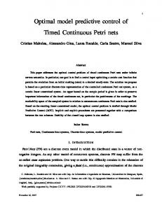
Fig. 2. Explicit representation of a discrete implicit differential transition.
In this work, the fundamental contribution is the unified Petri net-based representation of both parts of a hybrid dynamic system. Evidently, the main effort is to represent the continuous part in terms of Petri nets. To make design issues and procedures more transparent, we tried to deviate as little as possible from the concepts and tenets of ordinary Petri nets. Thus, we created our extension by making use of the principles established in the context of continuous Petri nets with maximal speeds depending on time [2], of hybrid Petri nets [9], and of dynamic Petri nets [19]. In our approach, the so-called “invariant phases” are equivalent to the integration step that would be used to numerically integrate the differential equations. The result is a new type of Petri net, which we call a differential Petri net (DPN), that is able to represent the continuous system part and the discrete-event system part of a hybrid system in a collective model. DPN’s are fully defined in Section II. In Section III, we present the evolution rules for DPN’s, while Section IV discusses their general properties and behavior. Section V contains an example along with a discussion of capabilities and issues related to DPN’s and is followed by the conclusion. II. DIFFERENTIAL PETRI NETS A first attempt to break through the barrier of representing only integer quantities within the Petri nets framework has been the continuous Petri net model [9]. There have been a number of continuous Petri net versions: 1) the constant speed; 2) the variable speed; and 3) the asymptotic continuous Petri nets. Their differences lie in the way the stream of events is approximated [3], [20]. In the case of the constant-speed continuous Petri nets (CCPN), each transition is associated with a constant maximal speed which cannot be changed; however, to represent, for example, some control objective, the maximal firing speed must depend on time. In this way, two extensions of CCPN have been defined, one in [13] called continuous Petri net with maximal speeds depending on time and another in [14] named controlled continuous Petri net. In these two models, the time function associated with continuous transitions can be varied. The above nets allowed only positive or null markings. Instead, the dynamic hybrid Petri net (DHPN) [19], which is a combination of a dynamic continuous Petri net with a discrete Petri net, has markings that can be positive or negative. DHPN has an incidence matrix that is in block diagonal form, facilitating the search for invariants. This Petri net extension permits us to model in a unified representation a hybrid system whose continuous part simply cooperates with a discrete-event part (as a supervisor). However, it does not allow us
to model a hybrid system where the continuous and the discrete parts are influencing each other’s evolution. A further difference with the model presented here is that the arc weights can only be positive. The above may create difficulties in the representation of common industrial controller functionalities. Having finished this brief review of various Petri nets related to the representation of continuous quantities, we define now a new class of Petri nets, which we call DPN. They possess the advantages of the continuous Petri nets with maximal speed depending on time, those of the DHPN’s and of course those of the regular Petri nets. Under the assumption that the continuous system can be represented by a finite number of linear first-order differential state equations, they are powerful enough to model a hybrid system in a single graph. A DPN is composed of: 1) discrete places and discrete transitions, just as in ordinary Petri nets and 2) differential places and differential transitions (symbolism in Fig. 1). To accommodate particular modeling needs, it is possible to include in DPN’s continuous places and continuous transitions [9]. In the same way as that in a DHPN, the marking of a differential place is a positive, negative, or null real, representing a state variable of the continuous system that is modeled. To every differential transition we associate a firing speed representing either a variable proportional to a state variable (or a marking of a differential place) or an independent variable. Since a differential transition is always enabled, to discretize the continuous system, we introduce to every differential transition a firing frequency representing the integration step that would be used when carrying out an integration of the differential equation. According to the Petri net theory, this delay is associated to the implicit discrete transition linked by a discrete place to this differential transition as shown in Fig. 2. The intrinsic characteristics associated to a differential transition do not allow the definition of autonomous DPN’s. In fact, inherent in the differential transition is the notion of time, permitting the discretized “view” of continuous systems with a certain period (namely, the integration step). Thus, a DPN is, by definition, a timed differential Petri net. A. Timed Differential Petri Nets—Definition of Structure
h
Ji
Definition 1: A timed differential Petri net is defined by B verifying the following conditions. ; with 1) R is a Petri net defined by R = P; T ;
R; f; M0 ;
• •
P T
h Pre Posti : finite set of places with j j 1 P : finite set of transitions with j j 1 T P
= n T