Sensors & Transducers, Vol. 172, Issue 6, June 2014, pp. 229-234
Sensors & Transducers © 2014 by IFSA Publishing, S. L. http://www.sensorsportal.com
Direct Adaptive Fuzzy Variable Structure Control Design without Sliding Mode for Nonlinear Systems with Unmatched Disturbances Xiaoyu Zhang North China Institute of Science and Technology, Yanjiao 206#, East Beijing, 101601, China Tel.: +86-10-61591487, fax: +86-10-61591487 E-mail:
[email protected]
Received: 11 April 20014 /Accepted: 30 May 2014 /Published: 30 June 2014 Abstract: Fuzzy adaptive sliding mode control method is a good way to resolve the control problem when the system mathematic model is unknown. However, reaching condition must be satisfied in this method. In this paper, a kind of fuzzy adaptive variable structure control method is presented in which sliding mode doesn’t exist in closed-loop system. Dynamic fuzzy logical system (DFLS) is introduced to form the variable structure controller (VSC) which parameters are self-tuned on-line. Then the stability of the closed-loop system is proved by using Lyapunov stability theories. The switching logic of the VSC is not determined by the sliding mode defined directly, and the reaching condition of the sliding mode is not required anymore. Robustness, chattering free and adaptive character can be obtained. Finally, simulation results on inverted pendulum are proposed to confirm the performance under perturbations. Copyright © 2014 IFSA Publishing, S. L. Keywords: Sliding mode, Fuzzy, Adaptive, Variable structure control.
1. Introduction Fuzzy adaptive sliding mode control in recent years is rapid developed and gradually perfected as one of the good techniques for uncertain systems. Its study tends to application research and control of many kinds of industrial plants [1-16]. According to different utilizations of the fuzzy logic system in the sliding mode control it can be divided into direct and indirect adaptive method. For example, Li Jichao presented the application of the indirect adaptive control method to the control system electric arc furnace [1], Liu Shanmei used direct adaptive control method in the control system of PMSM [2] and Dong Xiaomin apply direct adaptive method to the vehicle suspension system with time delay [4]. For additional example, in T. H. Ho’s research direct adaptive
http://www.sensorsportal.com/HTML/DIGEST/P_2129.htm
method is applied to the hydraulic transmission and control system [13], Shahraz utilized indirect adaptive control method in nonlinear chemical process control [16]. The above applications have achieved good control effect in industry. For the details described literature about fuzzy adaptive sliding mode control one may refer to [10]. Variable structure control (VSC) mainly includes two groups: One is VSC with sliding mode in which the control switches according to a pre-designed sliding mode manifold in order to drive the system state onto the manifold. It becomes the most popular kind of VSC due to its robustness to the matched disturbances. However, it needs satisfaction of reaching condition. The other VSC is that without sliding mode, which does not require the reaching condition of sliding mode.
229
Sensors & Transducers, Vol. 172, Issue 6, June 2014, pp. 229-234 Fuzzy adaptive control method itself contains adaptiveness to external disturbance and uncertainty. Therefore, if the adaptive laws and the control law guarantee the stability of the tracking error given the disturbance and uncertainty, the closed-loop system has enough robustness. Consequently, this paper uses dynamic fuzzy logic system (DFLS) for nonlinear function approximation, and then variable structure control without sliding mode is designed to guarantee that the tracking error is asymptotically stable by using Lyapunov stability theory. There is not sliding mode in the VSC and so not reaching conditions. The switching of the VSC is via tracking errors and robustness can still be achieved due to the adaptability of DFLS to uncertainties and external disturbance.
3. Dynamic Fuzzy Logic Systems As we know, fuzzy logic system has strong approximation ability. Its output is attached to a dynamic filters will form dynamic fuzzy logic system (Dynamic Fuzzy Logic Systems, DFLS). Lixin Wang studies a kind of DFLS in which the closed-loop system stability and the error convergence are validated [17]. J. X. Lee uses DAFLS to online approximation and control, thus adaptive controller is constructed based on it that has low-pass filtering function [18]. The similar analysis is also studied by Shitong Wang [19]. Using singleton fuzzifier, product inference rules and average defuzzifier method, a dynamic fuzzy logic system (DFLS) can be described as follows [18], gˆ ( x) = −ξ [ gˆ( x) − ΘT p ] ,
(4)
2. Problem Formulation Consider the nonlinear system with the form of x = Ax + b[ f ( x) + b( x)u + d ( x, t )] ,
(1)
where x = [ x1 , x2 , , xn ]T is the state vector, u (t ) is the control input, d ( x, t ) represents the unmatched disturbance and unmodelled dynamics, the constant matrices A, b are defined as 0 0 A= 0
1 0 0 0 , b = , 1 1 0 0
where g ( x ) is the nonlinear scalar function to be approximated, Θ = [θ1 ,θ 2 θ M ]T is the adjustable parameter of the DFLS which can be turned on-line by the adaptive laws, gˆ( x) is the approximation output. ξ > 0 is the real scalar to be designed, p( x) = [ p1 ( x ), p2 ( x), pm ( x)]T is the fuzzy basis function vector, M is the amount of fuzzy rules, H is the state vector dimension. Let parameters ahm , bhm depicted the membership functions of xh , then the fuzzy basis function is of the form H
pm ( x) =
with b ( x) is known upper bound function. The tracked model is
i=0
h=1 H
∏ μmh ( xh )
μ mh ( xh ) = exp[−(
, (5)
xh − a )] . bhm m h
The following lemma [17] is introduced for its later application. Lemma 1: For smooth nonlinear vector field g ( x) : R n → R , there is a parameter
n-1
x d = Ax d + b[-å ai x di+1 + r (t )] ,
M
m=1 h=1
and the nonlinear functions f ( x), b( x) are unknown but satisfy the following assumption. Assumption 1: f ( x ), b( x) are all bounded. Without loss of generality, b ( x) > b( x) > 0 holds
∏ μmh ( xh )
sup g ( x) − g * ( x) Θ* = arg min θ∈Ωθ , x∈Rn
(2)
where xd = [ xd1 , xd2 ,, xdn ]T is the tracked state, a0 , a1 , an−1 are Hurwitz coefficients, r (t ) is the tracked reference signal. Denote error vector
where g * ( x) is the approximation output of fuzzy logic system of DFLS (4), namely
e = [e1 , e2 , , en ]T ,
g * ( x) = Θ *T p .
ei = xi − xd
i
( i = 1, 2,, n ),
(3)
then the problem is to design fuzzy adaptive variable structure controller u (t ) so that the error vector e asymptotically stable.
230
to
guarantee ∀ε ∈ R, ε > 0 ,
g ( x) − g * ( x) < ε ,
(6)
The fuzzy inference rules of the fuzzy logic system are designed as follows. if x1 is a11 and x2 is a12 and …… xH is a1H then gˆ( x) is θ1 ,
Sensors & Transducers, Vol. 172, Issue 6, June 2014, pp. 229-234 if x1 is a12 and x2 is a22 and …… xH is aH2 then gˆ( x) is θ 2 , …… if x1 is a1M and x2 is a2M and …… xH is aHM then gˆ( x) is θ M . In the following SMC controller design, the DFLS described by (4) and the above rules of the fuzzy logic system are adopted directly for the approximation of unknown dynamics.
4. Controller Design For the system (1), it is convenient to attribute the unmatched disturbance and uncertainty factors into one nonlinear function approximation for identification with the form of g ( x) =
f ( x ) + [b( x) − b ( x)]u + d ( x, t ) . b ( x)
(7)
In this way a DFLS is constructed to approximate g ( x) which input vector is x = [ x1 , x2 , xn ]T . Afterwards, design the VSC controller as
controller (8) forms a complicated function. In next section the overall system stability will be analyzed.
5. Stability Analysis The main result is concluded as the following theorem. Theorem 1: For the nonlinear system (1) and the given tracked reference signal (2), the tracking error of the closed-loop system formulated by the fuzzy adaptive VSC (8-10) is asymptotically stable if the parameters λ j satisfy 1) λ j > 0,
j = 1, 2, n − 1 ,
λ1 0 2) D = 0 ±1
±1 ±1 0 λ3 ±1 > 0 . ±1 ±1 1
i =0
[ε h + kb ( x) e ]sgn en ,
(8)
V (t) =
−1
where the parameter k satisfies k > max λi + i =1,n −1
n +1 , 2
(9)
and the adaptive law is constructed as
0
λ2
0
Proof: It is easy to see that D = DT , D > 0 . Choose a Lyapunov function of the tracking error with the form of
n −1
u(t ) = −b −1( x) ai ydi + b −1( x)r(t ) − gˆ( x) −
0
α 2
1 1 T eT De + ( gˆ − ΘT p)2 + Θ GΘ , 2 2
= Θ * −Θ is the error between Θ and its where Θ corresponding optimal parameter Θ * . If D > 0, obviously V (t ) → ∞ when e → ∞ . Differentiating the Lyapunov function (11) with respect to time t one can get T p)( gˆ − ΘT p) + Θ T GΘ V (t ) = α ⋅ eT De + β ⋅ ( gˆ − Θ T = α [e2 , e3 en , en ] [λ1e1 ± en , λ2 e2 ± en
n
= α [G −1 ]T pb ( x) e , Θ i
n −1
i =1
gˆ ( x) = − β [ gˆ( x) − Θ P ] + α (1 + T
(11)
λn−1en−1 ± en , ci ei ± en ] +
(10)
i =1
T p)( gˆ − ΘT p) + Θ T GΘ . β ( gˆ − Θ
n
pT G −1 p )b ( x) ei i =1
with G ∈ R M ×M , G = G T , G > 0 , α > 0 , β > 0 all free positive matrix or scalars. In the equations (8) and (9), λi > 0 (i = 1, , n − 1) is optional argument to be designed, ε h > ε where ε = g ( x) − g * ( x) is the optimal approximation error. According to Lemma 1, the error ε can be small enough, thus ε h may be determined as arbitrary positive scalar by the situation of the system uncertainties and disturbances. The fuzzy adaptive VSC controller comprises of DAFLS approximator to gˆ( x) , Adaptive law, VSC controller and the reference signal. DAFLS is formulated by the equation (10-2) and the adaptive law is given by the equation (10-1). The VSC
n−1
n
i =1
i =1
Denote S a = (λi ei ei+1 ± ei+1en ) , Sb = ei . Then on account of that n −1
n−1
n−1
i =1
i =1
i =1
λi (ei − ei+1 ) 2 = λi (ei2 + ei2+1 ) − 2 λi ei ei+1 ≥ 0 n−1 n−1 1 max λi (ei2 + ei2+1 ) ≥ λi ei ei+1 i =1 2 i=1,n−1 i=1 n−1
max λi e ≥ λi ei ei+1 , 2
i =1,n −1
i =1
2 n n n−1 1 2 2 ≥ en ei+1 , ei ≥ ei2 , the e + ne n i =1 i =1 i=1 2 following inequality can be given,
and also
231
Sensors & Transducers, Vol. 172, Issue 6, June 2014, pp. 229-234 n +1 2 S a ≤ max λi + e , Sb ≥ e , 2 i=1,n−1
Substitute (10) into (12), one can get n −1
V (t ) = α ⋅ Sa + α ( ei + en )en − β [ gˆ( x) − ΘT p ][ gˆ( x) i =1
− ΘT p ] + α (1 + pT G −1 p)b ( x)[ gˆ( x) − n
ΘT p ] ei − α ⋅ pT G −1 pb ( x)[ gˆ( x) − i =1 n
n
i =1
i =1
where the system state vector x = θ θ with θ its pendulumangle excursion and u control voltage of the cart. It is estimated the upper bound function of nonlinear control gain b ( x ) as b (x ) = 280 , the controller is designed as (8), the other parameters α = β = 10 , ε = 0.01 , k = 10 , G = I are selected. The tracked model is set by T
(12)
1 0 0 xd = xd + r (t ) , −200 −30 200
ΘT p ] ei − α ⋅ b ( x)(Θ *T p − ΘT p) ei = α ⋅ S a + α ⋅ Sb sgn(en )en −
T
n
α ⋅ b ( x)[ g * ( x) − gˆ( x)] ei . i =1
Afterwards substitute the controller (8), one get V (t ) ≤ α ⋅ Sa + α ⋅ Sb sgn(en ) ⋅ en −
where xd = xd 1 xd 2 is the state of the tracked model, r (t ) is the reference signal. Let r (t ) = 0 , the control volt curve, angel excursion curve and its derivative curve of the inverted pendulum are shown in Fig. 1.
n
α ⋅ b ( x)[ g * ( x) − gˆ( x)] ei
The control input curve
i =1
0.035
≤ α ⋅ S a + α ⋅ Sb ⋅ b ( x)[ g( x) − gˆ( x) − (ε + kb −1( x) e ) sgn en ] −
0.03
n
0.025
The control volt /V: u
α ⋅ b ( x)[ g * ( x) − gˆ( x)] ei i =1
2
≤ α ⋅ (S a − k e ),
namely n +1 2 V (t ) ≤ α max λi + max ci e − i =1,n−1 i =1,n−2 2
{
}
0.02 0.015 0.01 0.005 0
(13)
-0.005
α k imin c e . =1,,n i 2
0
2
4
6
8
10
time /s
asymptotically stable by Lyapunov stability theories. The controller (8-10) is a kind of adaptive variable structure controller, in which dynamic fuzzy logic system is used as on-line approximation by (7). The reaching condition of sliding mode is no longer required to be satisfied by controller design. Even in the presence of strong interference, the uncertainties and unmodeled dynamics, the proof of Theorem 1 based on the controller is still valid, so the system also has strong robustness.
(a) The angle excursion and its derivative curves 0.15 θ
derivative of θ
0.1 θ and its derivative: rad, rad/s
Obviously, the derivative of Lyapunov function (11) is negative. V (t ) ≡ 0 if and only if e = 0 . That is, ∀e ∈ R n , e ≠ 0 , V (t ) ≠ 0 . Hence the overall system (1) is
0.05 0 -0.05 -0.1 -0.15 -0.2
0
2
4
6
8
10
time /s
6. Simulation
(b)
The inverted pendulum is a typical nonlinear, coupled system with disturbances, which mathematical model is of the form x1 = x2 , x2 = f ( x ) + b ( x ) u ,
232
(14)
Fig. 1. The control input curve and the angle excursion curves.
Consequently, r (t ) is set as square wave with 4 second period. The corresponding control volt curve,
Sensors & Transducers, Vol. 172, Issue 6, June 2014, pp. 229-234 angle excursion curve and the tracked state xd 1 are shown in Fig. 2. One can conclude that the tracking error converges quickly and the tracking effective is good. Finally, a pulse disturbance with unit magnitude value acts on the pendulum. Under the proposed controller in this paper, the control volt, the pendulum angle excursion curve and its angle speed
signal are shown in Fig. 3. From Fig. 1-3 it is shown that the proposed controller can guarantee the stability of the tracking error was verified by the above simulation results. Additionally, from these results the robustness and adaption ability to disturbance were also tested. As a result the proposed fuzzy adaptive VSC control without sliding mode is feasible. The angle excursion and its tracked signal 1.2
3
1 θ and its tracked signal: rad
The control volt /V: u
The control input curve 4
2 1 0 -1 -2
θ
tracked signal
0.8 0.6 0.4 0.2 0
0
2
4
6
8
-0.2
10
0
2
4
time /s
6
8
10
time /s
(a)
(b)
Fig. 2. The control volt and tracking signals when the reference signal is square wave.
The angle excursion and its derivative curves
The control input curve
1.5
0.1 θ
0
1 The control volt /V: u
θ and its derivative: rad, rad/s
derivative of θ
0.5
0
-0.1 -0.2 -0.3 -0.4 -0.5
-0.5 -0.6
-1
0
2
4
6
8
10
-0.7
0
2
4
(a)
6
8
10
time /s
time /s
(b)
Fig. 3. The control volt and angle excursion curves when disturbed.
7. Conclusions Through numerical simulation, it is shown that DFLS has not only strong robustness, but also a certain filtering function to unmodeled dynamics and disturbances, which thus greatly weakens the chattering of sliding mode control. The approximation capability of DFLS makes the system robust performance better and disturbance compensation ability strengthened. These guarantee the tracking performances. Therefore, in the absence
of sliding mode the reaching condition does not need to be required while in the overall closed-loop system fuzzy adaptive VSC is implemented.
Acknowledgements This work is supported by the National Natural Science Foundation of China (61304024), the Fundamental Research Funds for the Central Universities (3142013055), the Natural Science
233
Sensors & Transducers, Vol. 172, Issue 6, June 2014, pp. 229-234 Foundation of Hebei Province (F2013508110) and the Science and Technology plan projects of Hebei Provincial Education Department (Z2012089).
References [1]. J. C. Li, P. Guan, X. H. Liu, Application of indirect adaptive fuzzy sliding mode control in arc furnace, Journal of System Simulation, Vol. 21, Issue 2, 2009, pp. 542-546. [2]. S. M. Liu, Q. Ma, X. S. Chen, M. Wu, Application of adaptive fuzzy sliding mode controller in PMSM, Micromotors, Vol. 42, Issue 5, 2009, pp. 43-46. [3]. X. W. Zhang, F. Y. Wang, Study on adaptive fuzzy sliding mode control algorithm for the vehicle ABS, Automobile Technology, Vol. 32, Issue 10, 2009, pp. 25-30. [4]. X. M. Dong, M. Yu, C. Y. Liao, W. M. Chen, Adaptive fuzzy sliding mode control form magnetorheological suspension system considering nonlinearity and time delay, Journal of Vibration and Shock, Vol. 28, Issue 11, 2009, pp. 55-60+203. [5]. W. D. Gao, Y. M. Fang, W. L. Zhang, Z. Y. Fan, M. Wu, Application of adaptive fuzzy sliding mode control to servomotor system, Small & Special Electrical Machines, Vol. 37, Issue 11, 2009, pp. 32-36. [6]. J. P. Zhang, K. Liu, J. F. Lin, X. B. Ma, W. D. Yu, 4DOF adaptive fuzzy sliding mode control of excavator, Journal of Mechanical Engineering, Vol. 46, Issue 21, 2010, pp. 87-92. [7]. H. W. Wang, Y. W. Jing, C. Yu, Active queue management algorithm based on adaptive fuzzy sliding mode control, Journal of System Simulation, Vol. 20, Issue 23, 2008, pp. 6330-6332+6342. [8]. H. C. Zhao, J. M. Xu, D. Wang, Adaptive fuzzy sliding mode control for mass motion warhead, Journal of Tsinghua University (Science and Technology), Issue S2, 2008, pp. 1733-1736. [9]. Y. W. Peng, J. Chen, Z. F. Liu, M. Guo, Adaptive sliding mode control in chemical process application, Journal of Chemical Industry and Engineering (China), Vol. 63, Issue 9, 2012, pp. 2843-2850.
[10]. J. K. Liu, MATLAB Simulation for Sliding Mode Control, Tsinghua University Press, Beijing, 2005. [11]. Chih-Lyang Hwang, Hsiu-Ming Wu, Ching-Long Shih, et al, Fuzzy sliding mode under actuated control for autonomous dynamic balance of an electrical bicycle, IEEE Transactions on Control Systems Technology, Vol. 17, Issue 3, 2009, pp. 658-670. [12]. Wei Wang, Xiangdong Liu, Fuzzy sliding mode control for a class of piezoelectric system with a sliding mode state estimator, Mechatronics, Vol. 20, Issue 6, 2010, pp. 712-719. [13]. T. H. Ho, K. Ahn, Speed control of a hydraulic pressure coupling drive using an adaptive fuzzy sliding-mode control, IEEE/ASME Transactions on Mechatronics, Vol. 17, Issue 5, 2012, pp. 976-986. [14]. Her-Terng Yau, Cheng-Chi Wang, Chin-Tsung Hsieh, et al, Nonlinear analysis and control of the uncertain micro-electro-mechanical system by using a fuzzy sliding mode control design, Computers & Mathematics with Applications, Vol. 61, Issue 8, 2011, pp. 1912-1916. [15]. M. C. Zhu, Y. C. Li, Decentralized adaptive fuzzy sliding mode control for reconfigurable modular manipulators, International Journal of Robust and Nonlinear Control, Vol. 20, Issue 4, 2010, pp. 472-488. [16]. A. Shahraz, R. B. Boozarjomehry, A fuzzy sliding mode control approach for nonlinear chemical processes, Control Engineering Practice, Vol. 17, Issue 5, 2009, pp. 541-550. [17]. Lixin Wang, Design and analysis of fuzzy identifiers of nonlinear dynamic systems, IEEE Transactions on Automatic Control, Vol. 40, Issue 1, 1995, pp. 11-23. [18]. J. X. Lee, G. Vukovich, Identification of nonlinear dynamic system – A fuzzy logic approach and experimental demonstrations, in Proceedings of IEEE International Conference on Systems, Man and Cybernetics, Orlando, Florida, USA, 12-15 October 1997, pp. 1121-1126. [19]. Shitong Wang, Dongjun Yu, Error analysis in nonlinear system identification using fuzzy system, Journal of Software, Vol. 11, Issue 4, 2000, pp. 447-452.
___________________
2014 Copyright ©, International Frequency Sensor Association (IFSA) Publishing, S. L. All rights reserved. (http://www.sensorsportal.com)
234