1 DECEMBER 2002
HASHIZUME ET AL.
3379
Direct Observations of Atmospheric Boundary Layer Response to SST Variations Associated with Tropical Instability Waves over the Eastern Equatorial Pacific* HIROSHI HASHIZUME,1 SHANG-PING XIE,# MASATOMO FUJIWARA,@ MASATO SHIOTANI,@ TOMOWO WATANABE,& YOUICHI TANIMOTO,** W. TIMOTHY LIU,1 AND KENSUKE TAKEUCHI11 1 Jet Propulsion Laboratory, California Institute of Technology, Pasadena, California # International Pacific Research Center and Department of Meteorology, University of Hawaii, Honolulu, Hawaii @ Radio Science Center for Space and Atmosphere, Kyoto University, Kyoto, Japan & Tohuko National Fisheries Research Institute, Shiogama, Japan ** Graduate School of Environmental Earth Science, Hokkaido University, Sapporo, Japan 11 Frontier Observational Research System for Global Change, Yokosuka, Japan (Manuscript received 22 March 2002, in final form 11 June 2002) ABSTRACT Tropical instability waves (TIWs), with a typical wavelength of 1000 km and period of 30 days, cause the equatorial front to meander and result in SST variations on the order of 18–28C. Vertical soundings of temperature, humidity, and wind velocity were obtained on board a Japanese research vessel, which sailed through three fully developed SST waves from 1408 to 1108W along 28N during 21–28 September 1999. A strong temperature inversion is observed throughout the cruise along 28N, capping the planetary boundary layer (PBL) that is 1– 1.5 km deep. Temperature response to TIW-induced SST changes penetrates the whole depth of the PBL. In response to an SST increase, air temperature rises in the lowest kilometer and shows a strong cooling at the mean inversion height. As a result, this temperature dipole is associated with little TIW signal in the observed sea level pressure (SLP). The cruise mean vertical profiles show a speed maximum at 400–500 m for both zonal and meridional velocities. SST-based composite profiles of zonal wind velocity show weakened (intensified) vertical shear within the PBL that is consistent with enhanced (reduced) vertical mixing, causing surface wind to accelerate (decelerate) over warm (cold) SSTs. Taken together, the temperature and wind soundings indicate the dominance of the vertical mixing over the SLP-driving mechanism. Based on the authors’ measurements, a physical interpretation of the widely used PBL model proposed by Lindzen and Nigam is presented.
1. Introduction In the Tropics, surface wind and SST are tightly coupled and their interaction gives rise to rich space–time structures of the tropical climate and its variability (see Neelin et al. 1998 and Xie et al. 1999 for reviews). While it is well established that changes in tropical SST lead to changes in surface wind, the responsible mechanisms are often not well understood, partly because of insufficient observations over the remote tropical oceans. This paper presents results from direct obser* International Pacific Research Center Contribution Number 165 and School of Ocean and Earth Science Technology Contribution Number 6100. Corresponding author address: Dr. Hiroshi Hashizume, Jet Propulsion Laboratory, Mail Code 300-323, 4800 Oak Grove Drive, Pasadena, CA 91109-8099. E-mail:
[email protected]
q 2002 American Meteorological Society
vations of atmospheric response to slow SST variations associated with so-called tropical instability waves (TIWs) in the eastern equatorial Pacific. This section begins with a brief review of relevant literature and then demonstrates the importance of atmospheric vertical sounding. a. SLP driving vs vertical mixing Over warm ocean surfaces with SST higher than certain thresholds (say, 268–278C), deep adjustment that involves convection over the whole depth of the troposphere is often modeled as a single baroclinic mode without explicit treatment of the planetary boundary layer (PBL; Matsuno 1966; Gill 1980; Neelin and Held 1987; Xie et al. 1993). An alternative view of the pressure adjustment holds that pressure variations in the free troposphere is negligible and, instead, SST-induced air temperature variations within the PBL are the major cause of sea level pressure (SLP) variations that drive
3380
JOURNAL OF CLIMATE
surface flow over cool tropical regions where SSTs are below the convective thresholds (Lindzen and Nigam 1987). In reality, temperature variations in both the free troposphere and PBL contribute to those in SLP and hence surface wind in the Tropics (Wang and Li 1993; Chiang et al. 2001). In addition to the SLP driving for surface wind, Wallace et al. (1989) propose that vertical mixing of momentum near the surface is important in the eastern equatorial Pacific on seasonal, interannual, and longer timescales. A sharp SST front forms around 28N from June to December, separating the cold upwelled water on the equator from the warmer water (;278C) to the north. Wallace et al. hypothesize that when the southeasterly trade winds cross this equatorial front to warmer sea surface, vertical mixing intensifies, bringing fast-moving air down and thereby accelerating the surface flow. They suggest that the enhanced vertical mixing on the warmer side of the equatorial front is responsible for the maximum in meridional wind speed there.1 Paluch et al. (1999) describe their aircraft passage across the equatorial front: ‘‘The transition to the warmer sea surface was associated with a sudden appearance of numerous whitecaps (there were no whitecaps before this time), which suggests an increase in surface wind speed.’’ Making turbulence measurements on board the aircraft, Paluch et al. observe the intensity of eddy vertical velocity and hence vertical mixing increasing (decreasing) over the warm (cold) side of the SST front. In order for Wallace et al.’s (1989) mechanism to work, vertical shear with upward-increasing speed is required in the mean wind. Few vertical soundings of the atmosphere exist in the remote eastern Pacific. Dropsonde measurements were made in the equatorial Pacific during the First Global Atmospheric Research Program Global Experiment (FGGE) in spring 1979. An earlier version of FGGE data does not give wind readings below 900 mb (Kloesel and Albrecht 1989), while a recent analysis suggests an upward-decreasing wind shear in the eastern equatorial Pacific (Yin and Albrecht 2000), opposite to the shear required for the Wallace et al. mechanism. Analyzing soundings obtained in October and November 1989, Bond (1992) reports an upwardincreasing shear between the top of the mixed layer and sea surface that decreases north of the equatorial front, consistent with the Wallace et al. (1989) hypothesis. This difference in wind shear between the FGGE and Bond soundings may be due to seasonal variations in wind. Long-term wind profiler observations at the Galapagos Islands (0.98S, 89.618W) reveal a southerly jet at 400 m that intensifies during the colder half of the year (June–November) and weakens during the warmer half (December–May; Hartten and Gage 2000). Using soundings from September 1998, Anderson (2001) re1 An alternative advective mechanism is proposed by Tomas et al. (1999). See also Mahrt (1972).
VOLUME 15
ports that temperature is stably stratified to the south of the equatorial front while a mixed layer 500 m deep develops to the north. He further reports a rapid increase in surface wind speed as the ship crosses the front from the south. b. Tropical instability waves While the southward SLP gradient, with either linear (Lindzen and Nigam 1987) or nonlinear (Mahrt 1972; Tomas et al. 1999) PBL dynamics, contributes at least partially to the acceleration of the southerly winds across the equatorial front, the Wallace et al. (1989) vertical mixing mechanism appears dominant in monthly variability on the equatorial front (Hayes et al. 1989; Xie et al. 1998). During the colder half of the year (June–December), the equatorial front often displays large cusp-shaped meanders of typical periods of 1 month and typical zonal wavelengths of 1000 km (Legeckis 1977; Chelton et al. 2000), in association with oceanic TIWs that grow on shears of rapid equatorial currents (Philander 1978; Yu et al. 1995). Observations show coherent covariability in surface wind with amplitudes of 1–2 m s 21 . The southeasterly trades accelerate (decelerate) in the warm (cold) phase of the monthly SST waves, a phasing that is consistent with the vertical mixing mechanism but not with the Lindzen and Nigam (1987) SLP mechanism (Hayes et al. 1989). The latter would predict a 908 phase difference between wind and SST anomalies near the equator where the Coriolis effect is small. Global measurements of vector wind by satellite scatterometers allow the determination of space–time structure of TIW-induced wind variability, as demonstrated by Xie et al. (1998) with the European Remote Sensing scatterometer. Launched into space in June 1999, the SeaWinds scatterometer on the QuikSCAT satellite offers a higher space resolution and daily near-global coverage that can sample TIWs adequately. Applying various statistical technique to the QuikSCAT data, Liu et al. (2000), Chelton et al. (2001), and Hashizume et al. (2001) show that the trade wind acceleration is more or less in phase with SST variability, in support of the vertical mixing mechanism (see also Wentz et al. 2000; Thum et al. 2002). While buoy and satellite measurements both show the dominance of the vertical mixing mechanism for TIWinduced wind variability, it is unclear, physically, why the SLP mechanism should not be more important. Suppose that SST-induced changes in air temperature fill a 1-km-deep PBL as in Lindzen and Nigam (1987). A simple calculation to be presented in section 6 gives zonal wind anomalies ten times larger than observations. A tenfold reduction in the depth over which the SST effect on air temperature extends can bring the wind anomaly estimate closer to the observed amplitudes, but then the phase relative to SST still does not agree with observations.
1 DECEMBER 2002
HASHIZUME ET AL.
c. Vertical structure This influence depth of SST, though important for SLP adjustment, has never been observed directly. TIWs induce coherent changes in the amount of stratus clouds north of the equatorial front (Deser et al. 1993). While the cloud top is not determined in Deser et al. (1993), we suggest an influence depth of at least 400 m, the typical mixed-layer depth that often is also the cloud base (Kloesel and Albrecht 1989). This cloud response to TIWs is confirmed by a recent analysis of passive microwave measurements from the Tropical Rain Measuring Mission (TRMM) and Special Sensor Microwave Imager (SSM/I) satellites (Hashizume et al. 2001). Furthermore, Hashizume et al. (2001) detect coherent rainfall anomalies north of TIWs in the southern portion of the intertropical convergence zone (ITCZ), suggesting that the depth of the atmospheric response exceeds the PBL depth at least over the warm convective zone. The vertical structure of the atmosphere does not only hold the key to the puzzle of why the SLP mechanism is unimportant for the TIW phenomenon, but it can also provide direct evidence for the vertical mixing mechanism. Under the vertical mixing mechanism, we expect to see a couplet of wind acceleration and deceleration in the vertical as seen in a general circulation model simulation (Xie et al. 1998). In this model, SST-induced air temperature anomalies extend over a depth of 1 km and the SLP effect contributes equally to zonal wind anomalies as the vertical mixing, further indicating that there is no a priori reason why the SLP mechanism should be small. Vertical soundings of air temperature, humidity, and wind velocity were obtained along 28N from 1408 to 1108W in September 1999, on board the Japanese research vessel Shoyo-maru. This paper reports results from this cruise that cut across several SST waves on its way to the east. To our knowledge, this is the first time that the vertical structure of TIW-induced atmospheric waves has been measured. We use these in situ measurements to investigate the thermal and dynamic response of the atmosphere to the slow undulation of SST. The SST’s influence depth is a key parameter to dynamic adjustment as discussed above and will be a focus of this study. We show that the TIW effects penetrate the whole depth of the PBL, causing large vertical displacement of the temperature inversion that caps the PBL. Our wind velocity measurements indicate a vertical shear adjustment that is consistent with the Wallace et al. (1989) hypothesis. The observed thermal response is associated with greatly reduced pressure anomalies at the sea surface. The rest of the paper is organized as follows. Section 2 describes the cruise and measurements on board, which is followed by a brief analysis of satellite measurements that sample the Pacific both in space and time (section 3). Section 4 investigates the thermal response,
3381
and section 5 examines the vertical structure of wind velocity variability. Section 6 considers the vertical profile of pressure anomalies and addresses the question of why the SLP signal is smaller than one might expect. Section 7 is a summary. 2. Cruise data The equatorial Pacific was in a weak La Nin˜a state in 1999, with SST in the east slightly below the normal. TIW-induced SST waves started developing in late May, reached large amplitudes in June and July, and remained strong until the end of the year. On 16 September 1999, the research vessel Shoyo-maru of the Japan Fisheries Agency left Honolulu on its way to the equatorial Pacific. It arrived at 28N, 1408W on 21 September and began a week-long cruise along 28N, reaching 28N, 1108W on 28 September. We chose 28N for the survey because it is the latitude at which TIW-induced SST variance reaches a maximum (Hashizume et al. 2001). Encountering the strong south equatorial current that exceeded 1 m s 21 , the Shoyo-maru shifted its course slightly northward to 38N between 1108 and 1058W, and sailed farther northeastward thereafter to occupy stations for a squid fisheries survey (Fig. 1; Shiotani et al. 2000). Throughout the cruise, Vaisala RS-80 GPS radiosondes that measured air temperature, relative humidity, pressure, and wind velocity were launched four times a day. The sondes were released from a U-shaped wind screen made of strong vinyl on the rear deck of the Shoyo-maru, which was generally moving eastward (;6 m s 21 ) against the wind. During an intensive observation period that was centered on a cold cusp at 1258W, the launch frequency was increased to eight times a day. A total of 36 soundings launched between 1408 and 1058W are used in this study (Fig. 1). The soundings are binned at a 10-m vertical resolution using the linear interpolation. During the cruise, surface meteorological data were also measured at 1-min intervals. Continuous surface wind velocity and SLP measurements were made at 17and 10-m heights, respectively. SST were also continuously measured from the intake water at the bottom of the ship. Five-minute averages are shown in this paper for these surface measurements. Once every day, an ozonesonde (Science Pump ECC ozonesonde) was attached to the GPS radiosonde that measured ozone mixing ratio up to 25-km height. Details of ozone measurements and their results are presented in Shiotani et al. (2002). 3. Satellite measurements We use concurrent satellite measurements to supplement and put the Shoyo-maru survey into a large-scale perspective. Specifically, the TRMM Microwave Imager (TMI) makes measurements of SST through clouds ex-
3382
JOURNAL OF CLIMATE
VOLUME 15
FIG. 1. Sounding sites (triangle symbols) during the Shoyo-maru cruise from 16 Sep to 9 Oct 1999. Closed triangles (numbered from 1 to 36) refer to the sounding sites used in this paper. Superimposed is the TMI SST distribution averaged for 22–24 Sep. Heavy (light) shade denotes 238C , SST , 248C (248C , SST , 258C). The meanders of the equatorial front along 28N are caused by tropical instability waves.
cept under raining conditions and improves the sampling in cloudy regions as compared with traditional infrared radiometers (Wentz et al. 2000). We use a dataset for column integrated water vapor (WV) and cloud liquid water (CLW) derived by combining the TMI product and measurements by three co-orbiting (F-11, F-12, F14) SSM/Is (Hashizume et al. 2001). The original TMI and SSM/I data were processed at Remote Sensing Systems (Wentz, 1997) and obtained via FTP. The TMI and SSM/I data are originally gridded at a 0.258 3 0.258 and twice-daily resolution and we regridded them as 3day means at the 0.58 3 0.58 resolution. This 3-day averaging fills nearly all the oceanic grid points. The QuikSCAT wind velocity data are gridded by a successive correction method (Liu et al. 1998) at a 0.58 3 0.58 and twice-daily resolution. Both satellite and in situ measurements sample highfrequency atmospheric weather events such as the easterly waves that develop along the ITCZ. Taking advantage of the large disparity in typical wavelength between atmospheric easterly waves (;6000 km) and oceanic TIWs (;1000 km), we remove 128 moving averages in the zonal direction from satellite data to extract TIW signals. Hashizume et al. (2001) show that this highpass zonal filter removes weather noise quite effectively (their Fig. 3). A similar spatial filter of zonal moving average with a Gaussian-type weight (effective radius 58) is also applied to the radiosonde data along 28N. Hereafter, high-pass filtered variables are referred to as TIW-induced anomalies, or simply anomalies. Figure 2a shows the longitude–time section of highpass filtered TMI SST at 28N, with the straight solid line denoting the track of the Shoyo-maru cruise, which sampled three major SST waves between 1408 and 1108W. The typical amplitude of SST waves is 18C. TMI SST tracks the ship SST measurements quite well, par-
ticularly west of 1258W but showing a cold bias of 0.58– 18C to the east (Fig. 3b). The combined TMI and SSM/I data indicate that TIWs exert a clear influence over WV and to a lesser degree, over CLW (Figs. 2b,c). In order to further sharpen TIW signals, we make moving averages along the westward-propagating TIW phase line at each grid point for a 13-day period centered at the time of the Shoyomaru’s passage. The resultant composite distributions reinforce the notion that WV and CLW are largely in phase with SST (Fig. 2d), confirming the results of Hashizume (1998), Liu et al. (2000), and Hashizume et al. (2001). The longitude–time sections of high-pass filtered wind velocities also show a clear westward copropagation with SST (Figs. 2e,f). The 13-day composites reaffirm this association (Fig. 2g); both wind components are nearly in phase with local SST anomalies, but the maximum easterly anomaly tends to shift slightly to the east of the SST maximum, a phase difference Hashizume et al. (2001) attributed to SLP effects. The association between wind velocity and SST is quite apparent in the longitude–time sections based on satellite measurements. Detecting TIW signals becomes more difficult, however, with a one-time transect on board the Shoyo-maru, which contains high-frequency variability unrelated to TIWs. Figure 3a shows 5-min zonal wind speed measured on board the Shoyo-maru (solid line) that contains more variability than the satellite measurements. The Shoyo-maru and satellite measurements are similar on the TIW scale, except over the SST minimum centered at 1358W. The QuikSCAT captures the reduced wind speed over the 1258W SST minimum but shows little covariability with SST between 1228 and 1158W. Regarding the meridional wind veloc-
1 DECEMBER 2002
HASHIZUME ET AL.
3383
FIG. 2. Time–longitude sections of satellite measurements along 28N: (a) SST (8C), (b) columnintegrated water vapor (WV; mm), (c) cloud liquid water (CLW; mm), (e) zonal wind (U; m s 21 ), and (f ) meridional wind (V; m s 21 ). Positive values are shaded and the straight lines denote the Shoyo-maru cruise track. (d) The composite distribution of SST (8C; solid line), WV (mm; dashed line), and CLW (mm; dotted line) by moving average along the westward-propagating TIW phase line during 13 days before and after each point along the cruise line. (g) Same as (d) except for U (m s 21 ; dashed line) and V (m s 21 ; dotted line).
ity, the QuikSCAT data indicates few TIW signals on the Shoyo-maru track (Fig. 2f), partly because of the contamination by high-frequency weather noise (see appendix). For this reason, we will not discuss meridional wind variations further in this paper. 4. Thermal response to TIW-induced SST variations The following three sections analyze the Shoyo-maru survey data. The results will be related to satellite measurements where appropriate. We begin with temperature and humidity response. a. Basic vertical structure Tropospheric temperature generally decreases with height at a lapse rate between the dry adiabatic and moist adiabatic. A thin inversion layer where temperature increases with height often caps the PBL over cold ocean surface in the descending branch of the Hadley circulation (e.g., Hastenrath 1995). Such a temperature inversion is observed in all the Shoyo-maru soundings at 28N. It appears as a strongly stratified layer at 1–1.6 km in the cross section of virtual potential temperature along 28N (Fig. 4). The filled star symbols mark the inversion height (see the definition in the figure caption).
Figure 5a shows a sounding in the cross section. Above a hydrostatically unstable layer (;20 m deep) near the sea surface is a 400-m-deep mixed layer where both the virtual potential temperature (solid line) and specific humidity (dotted line) are constant in the vertical. Temperature becomes weakly stably stratified and specific humidity starts to decrease slightly, both indicative of a cloud layer from 500 m all the way to the inversion that is located at 1550 m in this particular sounding. The presence of clouds is further corroborated by high relative humidity (dashed line) up to 80%–90%. The sharp inversion, only 100 m thick, marks the cloud top, above which humidity decreases rapidly.2 Such a vertical structure—a thin unstable surface layer, a mixed layer topped by a cloud layer, and an inversion capping—is often observed in the eastern equatorial Pacific (Kloesel and Albrecht 1989; Bond 1992; Anderson 2001). b. Temperature From the Fig. 4 top, it is quite apparent that TIW’s influence reaches the full depth of the PBL. The mixed2 In the Tropics poleward of the ITCZ and the subtropics, cumulus clouds often rise above a weaker inversion over warm SSTs (e.g., Bretherton and Pincus 1995).
3384
JOURNAL OF CLIMATE
VOLUME 15
FIG. 3. (a) Surface zonal wind anomaly (m s 21 ). (b) SST anomaly (8C). Solid lines and open circles show the ship observation and the satellite observation, respectively.
layer temperature follows the SST, with its minima clearly locked to the cusps of TIWs. The inversion layer varies its height (star symbols) from 1000 to 1600 m, again following the underlying SST variations. For example, SST increases by 28C from 1368 to 1318W, and the inversion height increases by 300 m. In response to the SST minimum centered at 1258W, the inversion drops its height as much as 500 m. The correspondence between the inversion height and local SST is not perfect. Between 1238 and 1108W, the inversion height experiences one single depression (except a small dip at 1128W) while SST shows two waves. At 1158W, the inversion is lowered to 1000 m despite that the SST reaches a weak local maximum. A close look into the large-scale structure of the SST waves (Figs. 1 and 2a) suggests that the SST maximum at 1158W is short lived in a failed attempt at developing a second trough of the SST front within the major wave that spans 1238 and 1108W. In this sense, the lowered inversion height at 1158W can be viewed as a nonlocal atmospheric response to this major SST wave. In the mixed layer below 400 m, the effect of the secondary SST wave on air temperature is still clear with local maxima of air temperature and SST collocated. This suggests that the mixed layer responds to local SST changes while the height of the main PBL-capping inversion is controlled more by larger-scale SST waves. The sounding in Fig. 5a, obtained at the warm phase of TIWs, is characterized by a smooth transition from the mixed layer to a cloud layer above. At TIW’s cold phase (1158W), by contrast, the mixed layer is separated from the upper PBL by a weak, secondary inversion (Fig. 5b). Such a local maximum in static stability at the top of the mixed layer is commonly seen in the Shoyo-maru soundings over the colder sectors of TIWs (triangle symbols in Fig. 4). We define a secondary stable layer as the first level from the surface where virtual potential temperature increases by 0.5 K in a 100-m layer.
FIG. 4. (top) Longitude–height section of virtual potential temperature (K). The star symbol marks the main inversion defined as where virtual potential temperature gradient (evaluated over 100-m layers) is largest in the part of the atmosphere with specific humidity greater than 8 g kg 21 . The triangle symbol marks the secondary stable layer defined at the lowest level where virtual potential temperature increases by more than 0.5 K with a 100-m increase in height. (bottom) SST (8C) observed on board the Shoyo-maru. The numerals at the bottom denote the sounding numbers (see Fig. 1) and the shading marks nighttime.
Diurnal SST variations are small in this oceanic region, but the cloud-topped PBL can display significant diurnal cycle due to radiative forcing, with enhanced mixing and cloudiness in the predawn hours (Deser and Smith 1998; Ciesielski et al. 2001). However, the diurnal cycle does not seem to dominate our soundings. For example, we identified 14 soundings with a secondary stable layer at the top of the mixed layer. Among them, six were taken in day and eight at night (Fig. 4). Instead, the secondary stable layer almost never occurs over the warmer sector of TIWs but frequents the cold sector. c. Humidity and clouds Dry convection takes place in the mixed layer where temperature decreases with height rapidly at the adiabatic lapse rate. At the top of the mixed layer, the temperature cools down to a level that allows clouds to form. By releasing latent heat and emitting longwave radiation to space, these stratus clouds, capped by the main inversion, are the main agent for mixing above the mixed layer. At the warm phase of TIWs, the main inversion rises. In a thick layer between this inversion and mixed-layer top, relative humidity is high and virtual potential temperature increases slightly with height (Fig. 5a), both suggestive of the presence of clouds.
1 DECEMBER 2002
HASHIZUME ET AL.
3385
FIG. 5. Typical soundings over (a) warm and (b) cold SSTs during the Shoyo-maru survey: virtual potential temperature 2 295 (K; solid), relative humidity 310 21 (%; dashed), and specific humidity (g kg 21 ; dotted). The warm sounding was taken at 28N, 128.58W at 0526 UTC 24 Sep 1999 (sounding number 11 in Fig. 1), while the cold sounding was taken at 28N, 114.88W at 0527 UTC 27 Sep 1999 (sounding number 27).
At the cold phase of TIWs, by contrast, a stable layer (Fig. 5b) decouples the upper PBL from the mixed layer, shutting off the moisture supply from the sea surface. As a result, a large reduction of specific humidity is generally observed in this decoupled layer. Two relative humidity maxima occur, one at the mixed-layer top and one right beneath the main inversion. The former exceeds 80% and may allow a thin cloud layer to form at 300–400 m. The decoupled layer between the secondary (450 m) and main (1100 m) inversions is stably stratified. Relative humidity is generally lower than 80% in this decoupled layer and there are probably fewer clouds there than at TIW’s warm phase. This reduced radiative cooling at the base of the main inversion probably contributes to its diffusion at the cold phase of TIWs. Given that specific humidity drops by a factor of 2– 3 from within the PBL to above (Fig. 5), the large changes in the main inversion height conceivably modulate the vertically integrated water vapor content in the lower atmosphere. Figure 6a shows the longitude–height section of zonally high-pass filtered specific humidity anomaly along 28N. The dark shade indicates the positive anomalies above 2 g kg 21 . Most pronounced anomalies are located between 1000 and 1600 m, indeed associated with the vertical displacement of the main inversion. The vertically integrated water vapor content from the sea surface to 1600 m (solid curve in the middle panel) agrees quantitatively with satellite measurements (open circles) and is in phase with local SST variations. The breakdown of the vertical integration into the lower 1000 m and above shows that the variations between 1000 and 1600 m contribute the most. Water vapor changes in the lower 1000 m are smaller and not always consistent with local SST changes (dashed curve), pre-
sumably because the enhanced (weakened) vertical mixing acts against the effect of increased (reduced) surface evaporation over warmer (colder) SSTs. Thus, taken together, the Shoyo-maru and satellite measurements suggest that the column-integrated water vapor content is a good proxy for the inversion height near the equatorial front and may be used to monitor the vertical structure of the PBL in this region. 5. Wind response We now turn our attention to wind adjustment to changing SSTs. In general, wind velocity contains larger high-frequency fluctuations than temperature, relative to their respective means. Here we start with large-scale background wind structure, then examine wind variability on the TIW scale. a. Background structure Figure 7 shows the longitude–height sections of zonally low-pass filtered wind velocities, which may be taken as the background state in which the lower atmosphere makes adjustments to TIW-induced SST variations. Below 2000 m, the easterly velocity tend to increase toward the west, due to the large-scale SLP gradient associated with westward-increasing SST. In the zonal mean profile (Fig. 7a left), the easterly velocity reaches a maximum around the mixed-layer top, a tendency common throughout this low-pass filtered section. The southerly winds are confined within the PBL, reaching maximum speeds at or slightly above the mixedlayer top (Fig. 7b). Thus, our vertical soundings confirm Bond’s (1992) finding that both wind components increase speed with
3386
JOURNAL OF CLIMATE
VOLUME 15
(cold) phase by averaging soundings where the zonally high-pass filtered SST anomaly is above 0.58C (below 20.58C). There are 13 (9) soundings for the warm (cold) composite. Figure 8 shows the warm (cold) SST profile in solid (dashed) lines. The temperature and humidity composites confirm the results presented in section 4; namely, the main inversion rises trapping more moisture within the PBL over warmer SSTs. Note that humidity anomalies near the inversion significant contributes to virtual potential temperature anomalies (1 K for a humidity change of 6 3 10 23 kg kg 21 ). The overall structure of the zonal velocity composites for warm and cold SSTs are qualitatively similar, featuring a broad speed maximum between 300 and 700 m. Quantitatively, however, the wind shear is stronger both near the sea surface and above 1000 m in the cold SST composite as a result of reduced turbulent mixing. As TIWs cause SST to rise, the reduced static stability intensifies the mixing, leading to a weaker vertical shear. c. Intensive observing period
FIG. 6. (a) Longitude–height section of specific humidity anomalies (g kg 21 ). Positive values are shaded, with dark shades denoting anomalies greater than 2 g kg 21 . The main inversion and secondary stable layer are marked by star and triangle symbols (same as Fig. 4). (b) Vertically integrated water vapor (kg m 22 ) from the sea surface to 1600 m (solid line) and from sea surface to 1000 m (dashed line), with satellite-derived composite for column-integrated water vapor in open circles. (c) SST (8C) observed by the Shoyo-maru. The bottommost axis is the same as in Fig. 4.
height within the mixed layer (400–500 m). The variations in the vertical structure of temperature and humidity we discussed in the previous section further indicate variations in the strength of vertical mixing in response to SST waves. In particular, the formation of a stable layer that decouples the upper PBL from the mixed layer is indicative of reduced vertical mixing. This SST modulation of vertical mixing, along with the presence of vertical wind shear in the background state, provides circumstantial evidence for the vertical momentum mixing mechanism of Wallace et al. (1989) and Hayes et al. (1989). In search for direct evidence, the rest of this section examines wind profiles separately for the warm and cold phases of TIWs. b. Composites The moving averages of satellite measurements along the TIW phase line indicate that to the lowest order, easterly wind anomalies are in phase with SST (Fig. 2g). Here we make composite profiles for TIW’s warm
The Shoyo-maru cruised through a well-developed cold cusp that was centered at 1258W (Fig. 1). During a 30-h period, enhanced observations of this cusp were made, with radiosondes launched every 3 h. A total of 10 soundings were obtained during this intensive observation period (IOP) between 127.58 and 1228W. Both QuikSCAT and Shoyo-maru surface measurements capture the zonal wind modulation by this cold cusp (Fig. 3a). Figure 9 shows the soundings during the IOP. Four soundings (soundings 15–18) over cold SSTs display easterly wind shear of various degrees while the rest show little wind shear in the lowest 1000 m (soundings 13 and 19 are exceptions, with the former apparently contaminated by high-frequency fluctuations). Two most strongly sheared soundings (soundings 16 and 17) both feature strong temperature stratification above the mixed layer, indicative of suppressed vertical mixing. Such differences in temperature and wind velocity profiles between the warm and cold phases of TIWs are consistent with the vertical mixing mechanism of Wallace et al. (1989) and Hayes et al. (1989). 6. Pressure adjustment a. Sea level pressure Our in situ measurements show that the atmospheric response to TIW-induced SST variations extends to the top of the inversion height (;1.6 km). The hydrostatic SLP due to a 18C air temperature change within a 1000m surface layer is 0.4 hPa. Here, we assume a dry adiabatic lapse rate, which is a good approximation in the PBL (Fig. 5). With an effective drag coefficient for PBL depth mean zonal wind velocity e 5 0.56 days 21 (Deser 1993), the Coriolis force may be neglected at 28N be-
1 DECEMBER 2002
HASHIZUME ET AL.
FIG. 7. (left) Zonal mean vertical profile and (right) longitude–height section of the zonally low-pass filtered wind velocity: (a) zonal and (b) meridional wind (m s 21 ).
FIG. 8. Composite vertical profiles over warm (.0.58C; solid line) and cold (,20.58C; dotted line) SST anomalies: (a) virtual potential temperature (K), (b) specific humidity (g kg 21 ), (c) zonal wind velocity (m s 21 ), and (d) relative humidity (%). There are 13 (9) soundings for the warm (cold) composite.
3387
3388
JOURNAL OF CLIMATE
VOLUME 15
FIG. 9. (top) Longitude–height section of zonal wind velocity (vectors) and virtual potential temperature (K) (contours and shading) during the IOP. (bottom) SST (8C). The numerals with the plot refer to the number of the sounding site (see Fig. 1).
cause f /e 5 0.24 ( f is the Coriolis parameter). The equation for surface zonal velocity may be reduced to 2eU 5
1 dP . r dx
(1)
Here, the momentum mixing with the free atmosphere was neglected for simplicity, but the entrainment across the inversion may be important in the climatological balance of the mean boundary layer wind (Stevens et al. 2002). For a sinusoidal SST wave of an amplitude
of 18C, the amplitude of the zonal wind response is U ; 12 m s 21 , far too large compared to observations. Figure 10a shows the 5-min SLP measurements made on board the Shoyo-maru, which are dominated by semidiurnal and diurnal tides with amplitudes of about 2 hPa. We apply the harmonic analysis and remove the semidiurnal and diurnal harmonics. The resultant time series has a typical amplitude of 1.0 hPa at low frequencies (Fig. 10b). The tide-removed SLP, however, does not seem correlated with local SSTs. For example, no SLP increase is observed over any of the four SST minima between 1408 and 1108W, indicating that the SLP response to TIWs is much smaller than 0.4 hPa, the hydrostatic pressure due to a 18C temperature change within the PBL. The small SLP response is consistent with previous inferences based on buoy and satellite wind measurements (Hayes et al. 1989; Xie et al. 1998; Chelton et al. 2001; Hashizume et al. 2001). b. Vertical structure
FIG. 10. (a) 5-min sea surface pressure (SLP in hPa) measured by the Shoyo-maru along 28N. (b) SLP 2 1015 (hPa) with the diurnal and semidiurnal harmonics removed. (c) SST (8C).
Then what is responsible for the reduced SLP response? Figure 11a shows the longitude–height section of zonally high-pass filtered anomalies of virtual potential temperature. In addition to anomalies below 1000 m that are roughly of the same signs as the local SST anomalies, larger anomalies of the opposite signs are found further above between 1000–1600 m, which were not considered in our first attempt at SLP estimate. The latter anomalies are associated with the vertical displacement of the main PBL-capping inversion. Over warm SSTs, air temperature below the inversion increases via turbulent heat flux. At the same time, the main inversion rises (star symbols), leading to a strong
1 DECEMBER 2002
HASHIZUME ET AL.
3389
FIG. 12. Schematics of (left) temperature adjustment and (right) the resultant pressure anomaly profile, (a) observed in the Shoyomaru survey and (b) hypothesized in Lindzen and Nigam (1987). FIG. 11. (a) Longitude–height section of virtual potential temperature anomaly (K; shade .0). The main inversion and secondary stable layer are marked by star and triangle symbols (same as Fig. 4). (b) SST (8C). (c) The pressure difference (hPa) from 1600 to 1000 m (solid line), and from 1000 m to surface (dashed line). In (a) and (c), in addition to the high-pass filter described in section 3, the spatial filter of zonal three-point moving average with Gaussian-type weight (effective radius 18) is applied.
cold anomaly there. The same argument explains cold anomalies topped by warm ones over the cold phase of TIWs. Figure 11c displays hydrostatic pressure difference from 1600 to 1000 m (solid line) and from 1000 m to sea surface (dashed line). These hydrostatic pressure anomalies are both about 0.4 hPa in magnitude (in agreement with our earlier estimate), albeit with opposite signs. During the well-sampled IOP (127.58– 1208W), in particular, they nearly cancel each other. If we assume that the SST-induced pressure anomaly is negligible above the maximum inversion height, the SLP anomaly (their sum) is one order of magnitude smaller than hydrostatic pressure difference in either layer, a result consistent with our direct SLP measurements. This is consistent with satellite observations that show SLP-induced surface wind anomalies are small (Liu et al. 2000; Chelton et al. 2001; Hashizume et al. 2001). Figure 12a (right) is a schematic of temperature adjustment observed in the Shoyo-maru survey. An increase in SST causes a warming in the PBL and raises the inversion height to z 5 h w . If we assume that the SST-induced pressure anomaly is negligible above the
maximum inversion height, the temperature dipole establishes a pressure anomaly profile that peaks at the height of the original inversion (z 5 h c ) and then decreases monotonically downward (Fig. 12a right). The large pressure anomaly at z 5 h c can drive anomalous winds there. Figure 13 shows the scatterplot of zonal gradient of hydrostatic pressure difference from 1600 to 1000 m and zonal wind velocity averaged in 600– 1000 m. A correlation is apparent, suggesting a pressure gradient driving for wind in the upper PBL. This correlation also renders support to our inferred vertical profile of pressure anomaly. c. Back pressure effect Noting that SLP anomalies are too large in a PBL model of constant depth, Lindzen and Nigam (1987) propose a back pressure effect by allowing the PBL to adjust its height. In a broad sense, the reduced SLP anomalies observed in our measurements support this back pressure effect, but the responsible physical processes differ from their original hypothesis. Lindzen and Nigam (1987) use a constant lapse rate, assume a priori a vertical profile of perturbation air temperature of the same sign, and let the additional mass in a deepening PBL offset the SLP effect due to PBL warming, as shown schematically in the lower panels of Fig. 12. However, temperature anomaly profiles in our measurements are different from the one assumed in Lindzen and Nigam’s hypothesis. The PBL height change is still
3390
JOURNAL OF CLIMATE
FIG. 13. Scatterplot of zonal gradient of hydrostatic pressure difference from 1600 to 1000 m and zonal wind velocity averaged in 600–1000 m. There are two outliers.
crucial, not via additional mass in the boundary layer but by its temperature effect around the inversion height. In response to a surface warming, the deepening PBL generates a large cooling above the warming beneath, thereby reducing the pressure anomaly at the surface. Thus, we propose interpreting the back pressure effect as resulting from vertical displacement of the inversion and the dipole vertical structure of temperature anomalies (upper panels of Fig. 12). Our interpretation does not require the PBL top to be a constant pressure surface, an assumption made in the Lindzen–Nigam model. 7. Summary We have analyzed surface and radiosonde measurements obtained during the Shoyo-maru survey, which took place in the eastern equatorial Pacific for the 8day period of 21–28 September 1999. Between 1408 and 1058W along the equatorial front at 28N, three full wavelengths of TIWs were sampled with a total of 36 radiosondes. The typical range of TIW-induced SST variations was 38C during the survey. Our vertical soundings of temperature and humidity reveal, for the first time, that TIW influence reaches the full depth of the PBL. Throughout the survey, the PBL is capped by a strong temperature inversion that separates the moist air below from the dry one above. The height of this main inversion varies with TIWs, rising to 1500 m over warm SSTs and dropping down to only 1000 m over cold SSTs. This large vertical displacement of the main inversion causes vertically integrated water vapor content to increase (decrease) at the warm (cold)
VOLUME 15
phase of TIWs, a variation independently observed by satellites (Liu et al. 2000; Hashizume et al. 2001). At the TIW warm phase, a deep ‘‘cloud’’ layer (up to 1000 m) exists above the surface mixed layer, featuring weakly stable stratification, a gradual decrease of specific humidity and high relative humidity. At the cold phase, on the other hand, the upper PBL is decoupled from the mixed layer by a stable layer and becomes shallower and drier. Since the vertical displacement of the inversion-capped PBL height is the major cause of variations in column integrated water vapor, we suggest that this quantity, observable from satellites, may be used to monitor the inversion height within the equatorial cold tongue. Our analysis supports the vertical mixing mechanism for TIW-induced surface wind variability that is proposed by Wallace et al. (1989) and Hayes et al. (1989). The indirect evidence includes cruise mean profiles of zonal and meridional velocities that peak around the mixed layer top at 400–500 m, and marked changes in the inversion height and temperature and humidity stratification that are indicative of SST modulation of the strength and vertical extent of turbulent mixing. These results based on a zonal section are consistent with and complement the previously reported velocity (Bond 1992) and temperature (Anderson 2001) soundings along meridional sections across the equatorial front. Our wind velocity soundings further offer the first direct evidence for the Wallace et al. mechanism. Composite analysis reveals that over warm (cold) SSTs, the zonal wind shear increases (decreases) within the PBL, resulting in accelerated (decelerated) easterlies at the surface. The raw soundings during the well-sampled IOP corroborate this adjustment in wind shear. We caution, however, that this conclusion may be subject to the limited number of soundings that may not allow an unambiguous separation of TIW signals from higher-frequency noise. For example, we were not able to detect significant TIW signals in meridional wind velocity, a result that is contrary to statistical analysis of satellite measurements and may be due both to weather noise (see appendix) and to intraseasonal modulation of TIWs (Benestad et al. 2001). While surface wind measurements indicate that the vertical mixing is the leading mechanism (Hayes et al. 1989), it has never been clear why the SLP driving is not important as it is on larger spatial and longer temporal timescales (Deser 1993; Chiang and Zebiak 2000). Indeed, our direct measurements indicate that the TIW signal in SLP is one order of magnitude smaller than what one would expect from a warming/ cooling in an air column 1 km deep. The key to this SLP mystery lies in the vertical structure of SSTinduced temperature anomalies. In response to an increase in local SST, besides a warming in the lowest km, the rise of the inversion leaves a strong cooling in a layer between 1 and 1.6 km. The hydrostatic effects of this temperature dipole largely cancel each
1 DECEMBER 2002
3391
HASHIZUME ET AL.
other, leaving little pressure signal at the sea surface. In the upper PBL, by contrast, pressure anomalies reach a vertical maximum. We suggest that there, the pressure gradient force is indeed an important mechanism for TIW-induced wind variations. The above description of temperature and pressure adjustment observed in the Shoyo-maru survey offers a physical interpretation of the back pressure mechanism that Lindzen and Nigam (1987) hypothesize to reduce the SLP anomalies from what is expected from a PBL model of constant depths. While they assume a constant lapse rate and single-signed air temperature anomalies in the PBL, we suggest that the inversion and the dipole temperature anomalies in the vertical are at the heart of the back pressure effect. What remains unclear is the mechanism for the vertical displacement of the inversion: vertical mixing/entrainment or horizontal convergence? In our interpretation of the back pressure, we assumed that the SST-induced divergence/convergence and pressure anomalies are negligible at a vertical level above the PBL, which needs to be verified in future observations. Most of the World Ocean is not warm enough to support deep convection and the PBL-capping inversion is ubiquitous over the tropical oceans, a feature climate models have difficulty simulating due to insufficient resolution and inadequate representation of relevant physics.3 The lack of the inversion, which has a very small vertical scale, in a model will lead to an underestimate of temperature anomaly there and hence the back pressure in response to a SST change. Given this importance of the inversion for atmospheric adjustment, we call for an improved understanding and modeling of stably stratified PBL, in relation with large-scale dynamics and climate research. Acknowledgments. We would like to thank the Japan Fisheries Agency for providing the ship time, and Captain Kubota and the crew of the Shoyo-maru for their hospitality and assistance, without which this study would not have been possible. The contribution of W. Timothy Liu and part of the contribution by Hiroshi 3 The NCEP–NCAR reanalysis generally captures the salient climatological features. The eastern equatorial Pacific is an exception, where surface wind analysis is poor in the cold season (August– October) as compared to independent observations (Wu and Xie 2002).
Hashizume were performed at the Jet Propulsion Laboratory, California Institute of Technology, under contract with the National Aeronautics and Space Administration (NASA). The TMI and SSM/I data are obtained from the Web site of Remote Sensing Systems. This study is supported by the Ministry of Education, Fisheries Agency and Frontier Research System for Global Change of Japan, US NASA QuikSCAT and TRMM Missions, NOAA (NA17RJ1230) and NSF (ATM0104468). Graphic outputs were made by use of the GFDDENNOU Library, the GrADS, and the Mayura Draw. APPENDIX Synoptic Disturbances Pronounced weather disturbances are often observed in the eastern equatorial Pacific, in association with easterly waves (Chang 1970; Lau and Lau 1990; Raymond et al. 1998). They have a typical zonal wavelength of 6000 km and timescale of 5–10 days. Traveling westward, they have a much faster phase speed (;10 m s 21 ) than TIWs (;0.4 m s 21 ). Because of the large disparity in zonal scale from TIWs (;1000 km), high-pass zonal filtering is effective in removing these large-scale weather disturbances from TIWs (Hashizume et al. 2001), as is apparent by comparing Figs. 2 and A1. Such weather events were present during the Shoyomaru survey. In the surface zonal velocity field, the Shoyo-maru crossed a full wavelength of such weather disturbances and encountered weak (at 1408W), strong (1308W), and weak (1108W) easterlies on its way to the east. The daily NCEP–NCAR reanalysis at 850 hPa (Kalnay et al. 1996) indicates that these weather disturbances have a deep vertical structure, roughly in phase between the surface and above the PBL (Fig. A1; see also Lau and Lau 1990). The meridional wind disturbances appear to have higher frequencies than the zonal wind. As the Shoyo-maru sailed eastward at an average speed of 5 m s 21 , the Doppler-shifted wavelength for meridional wind was only 158 longitude, comparable to that of TIWs. The diminished difference in apparent wavelength between weather noise and TIWs may be responsible for the difficulty detecting meridional wind response to TIWs in the Shoyo-maru data. Because the weather disturbances feature a much larger zonal scale for zonal wind, we are able to separate them from TIW signals in the zonal velocity.
3392
JOURNAL OF CLIMATE
VOLUME 15
FIG. A1. Longitude–time section along 28N of wind velocity (m s 21 ) from (a) NCEP–NCAR reanalysis at 850 hPa and (b) twice daily QuikSCAT observations. The straight line approximately denotes the Shoyo-maru cruise line. For satellite observations, only zonally low-pass filtered data are shown.
REFERENCES Anderson, S. P., 2001: On the atmospheric boundary layer over the equatorial front. J. Climate, 14, 1688–1695. Benestad, R. E., R. T. Sutton, M. R. Allen, and D. L. T. Anderson, 2001: The influence of subseasonal wind variability on tropical instability waves in the Pacific. Geophys. Res. Lett., 28, 2041– 2044. Bond, N. A., 1992: Observations of planetary boundary-layer structure in the eastern equatorial Pacific. J. Climate, 5, 699–706. Bretherton, C. S., and R. Pincus, 1995: Cloudiness and marine boundary layer dynamics in the ASTEX Lagrangian experiments. Part I: Synoptic setting and vertical structure. J. Atmos. Sci., 52, 2707–2723. Chang, C. P., 1970: Westward propagating cloud patterns in the tropical Pacific as seen from time-composite satellite photographs. J. Atmos. Sci., 27, 133–138. Chelton, D. B., F. J. Wentz, C. L. Gentemann, R. A. de Szoeke, and M. G. Schlax, 2000: Satellite microwave SST observations of transequatorial tropical instability waves. Geophys. Res. Lett., 27, 1239–1242.
——, and Coauthors, 2001: Observations of coupling between surface wind stress and sea surface temperature in the eastern tropical Pacific. J. Climate, 14, 1479–1498. Chiang, J. C. H., and S. E. Zebiak, 2000: Surface wind over tropical oceans: Diagnosis of the momentum balance, and modeling the linear friction coefficient. J. Climate, 13, 1733–1747. ——, ——, and M. A. Cane, 2001: Relative roles of elevated heating and surface temperature gradients in driving anomalous surface winds over tropical oceans. J. Atmos. Sci., 58, 1371–1394. Ciesielski, P. E., W. H. Schubert, and R. H. Johnson, 2001: Diurnal variability of the marine boundary layer during ASTEX. J. Atmos. Sci., 58, 2355–2376. Deser, C., 1993: Diagnosis of the surface momentum balance over the tropical Pacific ocean. J. Climate, 6, 64–74. ——, and C. A. Smith, 1998: Diurnal variation of temperatures of the low-level wind and divergence fields. J. Climate, 11, 1730– 1748. ——, J. J. Bates, and S. Wahl, 1993: The influence of sea surface temperature on stratiform cloudiness along the equatorial front in the Pacific ocean. J. Climate, 6, 1172–1180.
1 DECEMBER 2002
HASHIZUME ET AL.
Gill, A. E., 1980: Some simple solutions for heat-induced tropical circulation. Quart. J. Roy. Meteor. Soc., 106, 447–462. Hartten, L. M., and K. S. Gage, 2000: ENSO’s impact on the annual cycle: The view from Galapagos. Geophys. Res. Lett., 27, 385– 388. Hashizume, H., 1998: Response of atmospheric boundary layer to tropical instability waves: Satellite scatterometer data analysis. M.Sc. dissertation, Hokkaido University, Sapporo, Japan, 24 pp. ——, S.-P. Xie, W. T. Liu, and K. Takeuchi, 2001: Local and remote atmospheric response to tropical instability waves: A global view from the space. J. Geophys. Res., 106, 10 173–10 185. Hastenrath, S., 1995: Climate Dynamics of the Tropics. Kluwer Academic, 488 pp. Hayes, S. P., M. J. McPhaden, and J. M. Wallace, 1989: The influence of sea surface temperature on surface wind in the eastern equatorial Pacific. J. Climate, 2, 1500–1506. Kalnay, E., and Coauthors, 1996: The NCEP/NCAR 40-year reanalysis project. Bull. Amer. Meteor. Soc., 77, 437–471. Kloesel, K. A., and B. A. Albrecht, 1989: Low-level inversions over the tropical Pacific—Thermodynamics structure of the boundary layer and the above-inversion moisture structure. Mon. Wea. Rev., 117, 87–101. Lau, K.-H., and N.-C. Lau, 1990: Observed structure and propagation characteristics of tropical summertime synoptic-scale disturbances. Mon. Wea. Rev., 118, 1888–1913. Legeckis, R., 1977: Long waves in the eastern equatorial Pacific: A view of a geostationary satellite. Science, 197, 1177–1181. Lindzen, R. S., and S. Nigam, 1987: On the role of sea surface temperature gradients in forcing low level winds and convergence in the tropics. J. Atmos. Sci., 44, 2418–2436. Liu, W. T., W. Tang, and P. S. Polito, 1998: NASA scatterometer provides global ocean-surface wind fields with more structures than numerical weather prediction. Geophys. Res. Lett., 25, 761– 764. ——, X. Xie, P. S. Polito, S.-P. Xie, and H. Hashizume, 2000: Atmospheric manifestation of tropical instability waves observed by QuikSCAT and Tropical Rain Measuring Mission. Geophys. Res. Lett., 27, 2545–2548. Mahrt, L. J., 1972: A numerical study of the influence of advective accelerations in an idealized, low-latitude, planetary boundary layer. J. Atmos. Sci., 29, 1477–1484. Matsuno, T., 1966: Quasi-geostrophic motions in equatorial areas. J. Meteor. Soc. Japan, 2, 25–43. Neelin, J. D., and I. M. Held, 1987: Modeling tropical convergence based on the moist static energy budget. Mon. Wea. Rev., 115, 3–12. ——, D. S. Battisti, A. C. Hirst, F.-F. Jin, Y. Wakata, T. Yamagata, and S. E. Zebiak, 1998: ENSO theory. J. Geophys. Res., 103, 14 261–14 290. Paluch, I. R., G. McFarquhar, D. H. Lenschow, and Y. Zhu, 1999: Marine boundary layers associated with ocean upwelling over the eastern equatorial Pacific ocean. J. Geophys. Res., 104, 30 913–30 936.
3393
Philander, S. G. H., 1978: Instabilities of zonal equatorial currents 2. J. Geophys. Res., 83, 3679–3682. Raymond, D. J., C. Lopez-Carrillo, and L. L. Cavazos, 1998: Casestudies of developing east Pacific easterly waves. Quart. J. Roy. Meteor. Soc., 124, 2005–2034. Shiotani, M., M. Fujiwara, S.-P. Xie, H. Hashizume, T. Saito, T. Watanabe, and F. Hasebe, 2000: SOWER/Pacific the Shoyo-maru Pacific ocean-atmospheric survey. SPARC Newslett., 14, 17–18 and II–III. ——, ——, F. Hasebe, H. Hashizume, H. Vo¨mel, S. J. Oltmans, and T. Watanabe, 2002: Ozonesonde observations in the equatorial eastern Pacific. The Shoyo-Maru survey. J. Meteor. Soc. Japan, 80 (4B), in press. Stevens, B., J. Duan, J. McWilliams, M. Munnich, and J. D. Neelin, 2002: Entrainment, Rayleigh friction, and boundary layer winds over the tropical Pacific. J. Climate, 15, 30–44. Thum, N., S. K. Ebensen, D. B. Chelton, and M. J. McPhaden, 2002: Air–sea heat exchange along the northern sea surface temperature front in the eastern tropical Pacific. J. Climate, 15, 3361– 3378. Tomas, R. A., J. R. Holton, and P. J. Webster, 1999: The influence of cross-equatorial pressure gradients on the location of nearequatorial convection. Quart. J. Roy. Meteor. Soc., 125, 1107– 1127. Wallace, J. M., T. P. Mitchell, and C. Deser, 1989: The influence of sea surface temperature on surface wind in the eastern equatorial Pacific: Seasonal and interannual variability. J. Climate, 2, 1492– 1499. Wang, B., and T. Li, 1993: A simple tropical atmosphere model of relevance to short-term climate variations. J. Atmos. Sci., 50, 260–284. Wentz, F. J., 1997: A well-calibrated ocean algorithm for special sensor microwave/imager. J. Geophys. Res., 102, 8703–8718. ——, C. Gentemann, D. Smith, and D. Chelton, 2000: Satellite measurements of sea surface temperature through clouds. Science, 288, 847–850. Wu, R., and S.-P. Xie, 2002: On equatorial Pacific surface wind changes around 1977: NCEP–NCAR reanalysis versus COADS observation. J. Climate, in press. Xie, S.-P., A. Kubokawa, and K. Hanawa, 1993: Evaporation-wind feedback and the organizing of tropical convection on the planetary scale. Part I: Quasi-linear instability. J. Atmos. Sci., 50, 3884–3893. ——, M. Ishiwatari, H. Hashizume, and K. Takeuchi, 1998: Coupled ocean-atmospheric waves on the equatorial front. Geophys. Res. Lett., 25, 3863–3866. ——, Y. Tanimoto, H. Noguchi, and T. Matsuno, 1999: How and why climate variability differs between the tropical Pacific and Atlantic. Geophys. Res. Lett., 26, 1609–1612. Yin, B., and B. A. Albrecht, 2000: Spatial variability of atmospheric boundary layer structure over the eastern equatorial Pacific. J. Climate, 13, 1574–1592. Yu, Z., J. P. McCreary, and J. A. Proehl, 1995: Meridional asymmetry and energetics of tropical instability waves. J. Phys. Oceanogr., 25, 2997–3007.