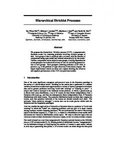
A gentle tutorial ... Dirichlet distribution, and Dirichlet Process introduction ..... ―A
Bayesian Analysis of Some Nonparametric Problems‖ Annals of Statistics.
Dirichlet Processes A gentle tutorial
SELECT Lab Meeting October 14, 2008
Khalid El-Arini
Motivation
We are given a data set, and are told that it was generated from a mixture of Gaussian distributions.
Unfortunately, no one has any idea how many Gaussians produced the data. 2
Motivation
We are given a data set, and are told that it was generated from a mixture of Gaussian distributions.
Unfortunately, no one has any idea how many Gaussians produced the data. 3
Motivation
We are given a data set, and are told that it was generated from a mixture of Gaussian distributions.
Unfortunately, no one has any idea how many Gaussians produced the data. 4
What to do? We can guess the number of clusters, run Expectation Maximization (EM) for Gaussian Mixture Models, look at the results, and then try again… We can run hierarchical agglomerative clustering, and cut the tree at a visually appealing level…
We want to cluster the data in a statistically principled manner, without resorting to hacks.
5
Other motivating examples Brain Imaging: Model an unknown number of spatial activation patterns in fMRI images [Kim and Smyth, NIPS 2006] Topic Modeling: Model an unknown number of topics across several corpora of documents [Teh et al. 2006] …
6
Overview Dirichlet distribution, and Dirichlet Process introduction Dirichlet Processes from different perspectives
Samples from a Dirichlet Process Chinese Restaurant Process representation Stick Breaking Formal Definition
Dirichlet Process Mixtures Inference
7
The Dirichlet Distribution Let We write:
P m Y ¡( k ®k ) ®k ¡1 P (µ1; µ2; : : : ; µm) = Q µk k ¡(®k ) k=1 Samples from the distribution lie in the m-1 dimensional probability simplex
8
The Dirichlet Distribution
Let
We write:
Distribution over possible parameter vectors for a multinomial distribution, and is the conjugate prior for the multinomial. Beta distribution is the special case of a Dirichlet for 2 dimensions. Thus, it is in fact a ―distribution over distributions.‖
9
Dirichlet Process
A Dirichlet Process is also a distribution over distributions. Let G be Dirichlet Process distributed: G ~ DP(α, G0) G0 is a base distribution α is a positive scaling parameter G is a random probability measure that has the same support as G0
10
Dirichlet Process
Consider Gaussian G0
G ~ DP(α, G0)
11
Dirichlet Process
G ~ DP(α, G0)
G0 is continuous, so the probability that any two samples are equal is precisely zero. However, G is a discrete distribution, made up of a countably infinite number of point masses [Blackwell]
12
Therefore, there is always a non-zero probability of two samples colliding
Overview
Dirichlet distribution, and Dirichlet Process introduction Dirichlet Processes from different perspectives
Samples from a Dirichlet Process Chinese Restaurant Process representation Stick Breaking Formal Definition
Dirichlet Process Mixtures Inference
13
Samples from a Dirichlet Process G ~ DP(α, G0) Xn | G ~ G for n = {1, …, N} (iid given G) Marginalizing out G introduces dependencies between the Xn variables
G
Xn N
14
Samples from a Dirichlet Process
Assume we view these variables in a specific order, and are interested in the behavior of Xn given the previous n - 1 observations.
Let there be K unique values for the variables:
15
Samples from a Dirichlet Process
Chain rule
P(partition)
P(draws)
Notice that the above formulation of the joint distribution does not depend on the order we consider the variables. 16
Samples from a Dirichlet Process
Let there be K unique values for the variables:
Can rewrite as:
17
Blackwell-MacQueen Urn Scheme
G ~ DP(α, G0) Xn | G ~ G Assume that G0 is a distribution over colors, and that each Xn represents the color of a single ball placed in the urn. Start with an empty urn. On step n:
With probability proportional to α, draw Xn ~ G0, and add a ball of that color to the urn. With probability proportional to n – 1 (i.e., the number of balls currently in the urn), pick a ball at random from the urn. Record its color as Xn, and return the ball into the urn, along with a new one of the same color. [Blackwell and Macqueen, 1973]
18
Chinese Restaurant Process
Consider a restaurant with infinitely many tables, where the Xn‘s represent the patrons of the restaurant. From the above conditional probability distribution, we can see that a customer is more likely to sit at a table if there are already many people sitting there. However, with probability proportional to α, the customer will sit at a new table.
Also known as the ―clustering effect,‖ and can be seen in the setting of social clubs. [Aldous] 19
Chinese Restaurant Process
20
Stick Breaking
So far, we‘ve just mentioned properties of a distribution G drawn from a Dirichlet Process In 1994, Sethuraman developed a constructive way of forming G, known as ―stick breaking‖
21
Stick Breaking
1. Draw X1* from G0 2. Draw v1 from Beta(1, α) 3. π1 = v1 4. Draw X2* from G0 5. Draw v2 from Beta(1, α) 6. π2 = v2(1 – v1) …
22
Formal Definition (not constructive)
Let α be a positive, real-valued scalar Let G0 be a non-atomic probability distribution over support set A If G ~ DP(α, G0), then for any finite set of partitions of A:
A1
23
A2 A3
A4
A5
A6
A7
Overview
Dirichlet distribution, and Dirichlet Process introduction Dirichlet Processes from different perspectives
Samples from a Dirichlet Process Chinese Restaurant Process representation Stick Breaking Formal Definition
Dirichlet Process Mixtures Inference
24
Finite Mixture Models
A finite mixture model assumes that the data come from a mixture of a finite number of distributions. α
π ~ Dirichlet(α/K,…, α/K) G0
π
cn ~ Multinomial(π)
Component labels
ηk ~ G0
η*k
cn
k=1…K
yn n=1…N 25
yn | cn, η1,… ηK ~ F( · | ηcn)
Infinite Mixture Models
An infinite mixture model assumes that the data come from a mixture of an infinite number of distributions α
π ~ Dirichlet(α/K,…, α/K) π
G0
cn
η*k
cn ~ Multinomial(π) ηk ~ G0 k=1…K
Take limit as K goes to ∞
yn n=1…N 26
yn | cn, η1,… ηK ~ F( · | ηcn)
Note: the N data points still come from at most N different components [Rasmussen 2000]
Dirichlet Process Mixture G0
countably infinite number of point masses
G α draw N times from G to get parameters for different mixture components
ηn
If ηn were drawn from, e.g., a Gaussian, no two values would be the same, but since they are drawn from a Dirichlet Process-distributed distribution, we expect a clustering of the ηn
yn n=1…N 27
# unique values for ηn = # mixture components
CRP Mixture
28
Overview
Dirichlet distribution, and Dirichlet Process introduction Dirichlet Processes from different perspectives
Samples from a Dirichlet Process Chinese Restaurant Process representation Stick Breaking Formal Definition
Dirichlet Process Mixtures Inference
29
Inference for Dirichlet Process Mixtures
Expectation Maximization (EM) is generally used for inference in a mixture model, but G is nonparametric, making EM difficult
G0 G α
ηn
Markov Chain Monte Carlo techniques [Neal 2000] Variational Inference [Blei and Jordan 2006] 30
yn n=1…N
Aside: Monte Carlo Methods [Basic Integration]
We want to compute the integral,
where f(x) is a probability density function. In other words, we want Ef [h(x)]. We can approximate this as:
where X1, X2, …, XN are sampled from f. By the law of large numbers, 31
[Lafferty and Wasserman]
Aside: Monte Carlo Methods [What if we don’t know how to sample from f?]
Importance Sampling Markov Chain Monte Carlo (MCMC)
Goal is to generate a Markov chain X1, X2, …, whose stationary distribution is f. If so, then
N 1 X p h(Xi) ¡! I N i=1 (under certain conditions) 32
Aside: Monte Carlo Methods [MCMC I: Metropolis-Hastings Algorithm]
Goal: Generate a Markov chain with stationary distribution f(x) Initialization:
Let q(y | x) be an arbitrary distribution that we know how to sample from. We call q the proposal distribution. A common choice Arbitrarily choose X0.is N(x, b2) for b > 0
Assume we have generated Xi+1:
If q is symmetric, X0, X1, …, Xi. To generate simplifies to:
Generate a proposal value Y ~ q(y|Xi) Evaluate r ≡ r(Xi, Y) where:
Set:
with probability r with probability 1-r
33
[Lafferty and Wasserman]
Aside: Monte Carlo Methods [MCMC II: Gibbs Sampling]
Goal: Generate a Markov chain with stationary distribution f(x, y) [Easily extendable to higher dimensions.] Assumption:
We know how to sample from the conditional distributions fX|Y(x | y) and fY|X(y | x) If not, then we run one iteration
Initialization:
Arbitrarily choose X0,Y0.
of Metropolis-Hastings each time we need to sample from a conditional.
Assume we have generated (X0,Y0), …, (Xi,Yi). To generate (Xi+1,Yi+1): 34
Xi+1 ~ fX|Y(x | Yi) Yi+1 ~ fY|X(y | Xi+1) [Lafferty and Wasserman]
MCMC for Dirichlet Process Mixtures [Overview]
We would like to sample from the posterior distribution: P(η1,…, ηN | y1,…yN) If we could, we would be able to determine:
how many distinct components are likely contributing to our data. what the parameters are for each component.
[Neal 2000] is an excellent resource describing several MCMC algorithms for solving this problem.
35
We will briefly take a look at two of them.
G0
G α
ηn
yn n=1…N
MCMC for Dirichlet Process Mixtures [Infinite Mixture Model representation]
MCMC algorithms that are based on the infinite mixture model representation of Dirichlet Process Mixtures are found to be simpler to implement and converge faster than those based on the direct representation. Thus, rather than sampling for η1,…, ηN directly, we will instead sample for the component indicators c1, …, cN, as well as the component parameters η*c, for all c in {c1, …, cN}
36
α π
G0
cn
η*k k=1…∞
yn n=1…N
[Neal 2000]
MCMC for Dirichlet Process Mixtures [Gibbs Sampling with Conjugate Priors]
Assume current state of Markov chain consists of c1, …, cN, as well as the component parameters η*c, for all c in {c1, …, cN}. To generate the next sample: 1. For i = 1,…,N:
If ci is currently a singleton, remove η*ci from the state. Draw a new value for ci from the conditional distribution: for existing c for new c
37
If the new ci is not associated with any other observation, draw a value for η*ci from: [Neal 2000, Algorithm 2]
MCMC for Dirichlet Process Mixtures [Gibbs Sampling with Conjugate Priors] 2.
For all c in {c1, …, cN}:
Draw a new value for η*c from the posterior distribution based on the prior G0 and all the data points currently associated with component c:
This algorithm breaks down when G0 is not a conjugate prior. 38
[Neal 2000, Algorithm 2]
MCMC for Dirichlet Process Mixtures [Gibbs Sampling with Auxiliary Parameters]
Recall from the Gibbs sampling overview: if we do not know how to sample from the conditional distributions, we can interleave one or more Metropolis-Hastings steps.
We can apply this technique when G0 is not a conjugate prior, but it can lead to convergence issues [Neal 2000, Algorithms 5-7] Instead, we will use auxiliary parameters.
Previously, the state of our Markov chain consisted of c1,…, cN, as well as component parameters η*c, for all c in {c1, …, cN}. When updating ci, we either:
choose an existing component c from c-i (i.e., all cj such that j ≠ i). choose a brand new component.
39
In the previous algorithm, this involved integrating with respect to G0, which is difficult in the non-conjugate case.
[Neal 2000, Algorithm 8]
MCMC for Dirichlet Process Mixtures [Gibbs Sampling with Auxiliary Parameters]
When updating ci, we either:
choose an existing component c from c-i (i.e., all cj such that j ≠ i). choose a brand new component.
Let K-i be the number of distinct components c in c-i. WLOG, let these components c-i have values in {1, …, K-i}. Instead of integrating over G0, we will add m auxiliary parameters, each corresponding to a new component independently drawn from G0 : [η*K +1 , …, η*K-i +m ] -i
Recall that the probability of selecting a new component is proportional to α.
40
Here, we divide α equally among the m auxiliary components.
[Neal 2000, Algorithm 8]
MCMC for Dirichlet Process Mixtures [Gibbs Sampling with Auxiliary Parameters]
2
1
2
1
α/3
α/3
α/3
η*1
η*2
η* 3
η*4
η*5
η* 6
η*7
Probability: (proportional to)
Components:
Each is a fresh draw from G0
Data:
y1
y2
y3
y4
y5
y6
y7
cj:
1
2
1
3
4
3
?
This takes care of sampling for ci in the non-conjugate case. A Metropolis-Hastings step can be used to sample η*c.
See 41
Neal‘s paper for more details.
[Neal 2000, Algorithm 8]
Conclusion
We now have a statistically principled mechanism for solving our original problem.
This was intended as a general and fairly high level overview of Dirichlet Processes. 42
Topics left out include Hierarchical Dirichlet Processes, variational inference for Dirichlet Processes, and many more. Teh‘s MLSS ‗07 tutorial provides a much deeper and more detailed take on DPs—highly recommended!
Acknowledgments
Much thanks goes to David Blei. Some material for this presentation was inspired by slides from Teg Grenager, Zoubin Ghahramani, and Yee Whye Teh
43
References David Blackwell and James B. MacQueen. ―Ferguson Distributions via Polya Urn Schemes.‖ Annals of Statistics 1(2), 1973, 353-355. David M. Blei and Michael I. Jordan. ―Variational inference for Dirichlet process mixtures.‖ Bayesian Analysis 1(1), 2006. Thomas S. Ferguson. ―A Bayesian Analysis of Some Nonparametric Problems‖ Annals of Statistics 1(2), 1973, 209-230. Zoubin Gharamani. ―Non-parametric Bayesian Methods.‖ UAI Tutorial July 2005. Teg Grenager. ―Chinese Restaurants and Stick Breaking: An Introduction to the Dirichlet Process‖ R.M. Neal. Markov chain sampling methods for Dirichlet process mixture models. Journal of Computational and Graphical Statistics, 9:249-265, 2000. C.E. Rasmussen. The Infinite Gaussian Mixture Model. Advances in Neural Information Processing Systems 12, 554-560. (Eds.) Solla, S. A., T. K. Leen and K. R. Müller, MIT Press (2000). Y.W. Teh. ―Dirichlet Processes.‖ Machine Learning Summer School 2007 Tutorial and Practical Course. Y.W. Teh, M.I. Jordan, M.J. Beal and D.M. Blei. ―Hierarchical Dirichlet Processes.‖ J. American Statistical Association 101(476):1566-1581, 2006.
44