In many applications of 2D digital image processing, discrete approximations of the MAT ..... The points of MAc(O) can be classi ed as CI (points with tangent continuity) ...... 4th International Conference Visualization in Biomedical Comput-.
Discrete Medial Axis Transform for Discrete Objects Anna Puig Puig
1 Introduction The Medial Axis Transform MAT was de ned by Blum in [Blu67] as an alternate description of the shape of an object. The MAT is the closure of the set of centers of maximal balls which can t inside the object. A ball is maximal if it is not contained by any other such ball. This model is homotopic with the object characteristics and it is continuous if the object is path-connected ([SPW96]). It is a unique and a complete model representation. In addition, it provides dimensionality reduction, symmetry detection and invertibility. Thus, it is an alternate compressed representation of objects and it preserves their topological characteristics. This is the reason why this description has been shown to be useful in CAD designs in order to reduce the computational complexity of certain algorithms. Nevertheless, it is a not minimal scheme and it is sensitive to small changes on the boundary of the object. Moreover, progress on its use has been limited by the di�culty of developping a robust, accurate and e�cient algorithm for its construction. In many applications of 2D digital image processing, discrete approximations of the MAT, such as skeletal representations, are used as decompositions of discrete objects whose width is not negligible and may vary. The main construction algorithms of these skeletons are thinning ([LLS92], [CCS95], [KSKB95], [LKC94]) and morphological methods ([MMD96]). These skeletons are continuous but they do not re ect all the topological features of the discrete objects and they are not complete representation schemes. Other skeletal schemes are based on Distance Map transformations (DM) extrapolating Blum's de nition to the discrete case ([Dan80], [KSKB95]). These skeletons constitute complete representation models but they do not preserve the connectivity of the axis in order to nd a minimal and compressed scheme representation ([ND97]). Even though the compression is a goal to attain, the preservation of the connectivity is essential to keep up the topological characteristics of the object boundary in order to apply algorithms such as those that realize pattern recognition directly on the skeleton instead of on the object boundary. Furthermore, as computing the distance from a pixel to a set of feature pixels is essentially a global operation, these algorithms are based on full scans of the images and, thus, their computational cost is proportional to the 1
size of the image. In this report, a Discrete Medial Axis de nition is proposed as a direct extension of Blum's de nition in order to achieve a complete and compressed model representation of discrete objects which retains the signi cant features of the object without introducing distorsions of its own. Moreover, it preserves the axis connectivity and it is based on local properties of the Distance Map which enable to design a seed algorithm for its construction whose cost is linear with the size of the object. First, in section 2, some de nitions and properties are reviewed. In section 3, the Discrete Medial Axis Transform for 2D discrete objects is de ned and its main properties are demonstrated. The algorithm of the MATD construction is proposed in section 4 and its evaluation and some simulations are analyzed in sections 5 and 6 respectively. The 3D-extension of the de nition and of the algorithm is discussed in section 7. Finally, the conclusions and the future work are presented in section 8.
2 De nitions and review Before the de nition of the Discrete Medial Axis Transform, it is necessary to state brie y some important de nitions of basic concepts from digital topology and some hypothesis about the initial digital objects. Let 0; Yh > 0g where Xl , Yl , Xh i Yh are the minimum and maximum values of the coordinates respectively. The borders of an image are considered as: border(I) = fpij = i = Xl k i = Xh k j = Yl k j = Yh g and it is assumed that 8pij 2 border(I); (pij ) = 0. Let O be a discrete object on an image I represented by a 8-connected set of pixels ([KR89]) such that its (pij ) = 1, then the boundary of the object on the image is: 2
boundary(O) = fpij =pij 2 O such that (pij ) = 1 & 9pi j : (pi j ) = 0 such that pi j 2 8neighbour(pij )g 0
0 0
0
0
0
Moreover, two object pixels are adjacents only if they are 8-adjacent and two non-object pixels are adjacent only if they are 4-adjacent. This statement avoids ambiguities in the classi cation of a pixel as interior or exterior to the digital object ([KR89]). There are various discrete distance functions in the discrete space which approximate the continuous euclidian metric. Not all of these metrics de ne distances in mathematical sense, as they do not full l the triangular inequality. With any of these distance functions, the distance from a pixel pij to a pixel set C can be considered as: dist(pij ; C) = minimump 2C fdist(pij ; pi j )g Def 1. The distance map of an image, I, referred to an object, O is the function: DM : I ! 5, is ( 5=2 ? 1) � M. � Chamfer distance: The local distances at a 4-neighbourpand at a 8-neighbour are the real numbers d1 and d2. If d1 = 1 and d2 = 2, the upper limit of the di�erence p p with the Euclidean distance in an (M + 1) � (M + 1) area is ( 2 2 ? 2 ? 1) � M. There are best approximations of the Euclidean distance such as d1 = 1 and d2 < 2 and there are good integer approximations which set d1 to 2 and d2 to 3. � Euclidean distance [Dan80]: distE (px0 ;y0 ; px1;y1 ) = (fabs(x1 ? x0); fabs(y1 ? y0 )) Dt (pij ) = fpi+h j +k =h2 + k2 � t2 g This metric gives the exact distance but two integer values must be stored for each pixel.
(a)
(b)
(c)
(d)
Figure 1: Di�erent neighbourhood shapes, radius 6 units: (a) City-block, (b) Chessboard, (c) Chamfer Distance and (d) Euclidean Distance. The above de ned metrics use di�erent pixel neighbourhoods that approximate, more o less accurately, the shape of a continuous euclidean disk. Figure 1 shows the di�erents shapes of the disks according to the metric used.
Proposition 1. The discrete skeleton computed with any discrete metric (nneighbours, chamfer and euclidean distance) is not always connected.
The examples shown in Figure 2 illustrate the above proposition. The fact that the skeleton is not connected disables continuous traversals of the structure along it. In particular, its computation must be based on a global scan 4
(a) city-block
(b) chessboard
(c) euclidian
Figure 2: Skeletons computed with di�erent metrics. of the image and it is not possible to perform a local strategy which would have a lower computational cost. It must be considered that these disconnections are not bounded by a neighbourhood instead, they may appear in cases such as of Figure 3.
Figure 3: Non bounded disconnections with the Euclidean metric. In order to avoid some of these problems, ([SGP96], [SGP93]) have proposed a continuous box-skeleton for discrete objects which preserves the homotopy, which does not have interior and whose shape is an abstract shape of the object. However, this skeleton does not converge to the Euclidean skeleton. Next, an euclidian skeletal de nition based on the Distance Map is proposed. It does not present discontinuities, it preserves the topological information and it is a complete representation scheme.
3 Discrete Medial Axis Transform Before presenting the theory in the rest of section 3, the main underlying ideas are rst outlined. This will hopefully help to better understand the motivation for the mathematics (see Figure 4). Let O be a continuous object of = dist((x; y) � �; bound(O))g The points of MAc (O) can be classi ed as CI (points with tangent continuity) and CII (points without tangent continuity) (see [Ver94]). Thus, MAc (O) is composed by the union of segments limited by CII points. All of these segments de ne a set of points which are centers of maximal disks inscribed into the 6
object. These centers can be clustered in pairs such that their associated disks have a non-empty intersection area (see Figure 5). CII points d2
CI points
d1
Center of disks Disks d1 and d2 Intersection of d1 and d2
Figure 5: MAc (O) with CI and CII points. It is possible to assume, without loss of generality, that the Continuous Medial Axis between every pair of inscribed maximal disks, D1 (px1 y1 ) and D2 (Px2 y2 ) is equivalent to the Continuous Medial Axis of the object which is de ned by the union of these pairs of disks D1 (px1 y1 ) [ D2 (px2 y2 ). For this reason, the general case of any discrete object may be reduced to the discretization of a continuous object Ou de ned as the union of two intersecting disks, non enclosed one into each other, of centers (x1; y1) and (x2 ; y2) respectively and of radii ra and rb. The following considerations must be taken into account:
� One continuous disk is discretized in the integer space using the Euclidean
metric, as a set of one or more discrete disks. In section 3.2, the relationships between the disks of the two spaces are analyzed. � The discretization of the metric produces that some tangencies between continuous disks change in the discrete metric. New discrete tangencies concepts are de ned in section 3.3. � The pixels of the discretization of the medial axis of the continuous object Ou full l some tangency properties between the disk and the boundary of the object. This case is analyzed in section 3.4.
3.2 Relationships between continuous disks and discrete disks In this section, the discretization of the continuous space and of the continuous metric is analyzed in order to de ne the relationships between the continuous and the discrete disks. The space R2 of the continuous object O and its Continuous Medial Axis MAc (O) is discretized in Z 2 . The center of a disk can be interior to a pixel, on an edge of the pixel or on one of its vertices (see Figure 6). The distance between the center of thep disk and the center of the pixel is labelled as d and it is bounded by 0 � d � 22 . The distance of each point of every pixel is collapsed to the distance of the center of the pixel. The error introduced in this process is �1 = d. 7
d
d
d
Figure 6: Locus of a point in relation to a pixel. The distance values associated to the centers of the pixels are discretized by the Euclidian Distance ([Dan80]). This new labelling produces an error �2 = DM(r) ? r. The Euclidean Distance can be expressed as: DM(r) = minimumd fd2 = x2 + y2 = r � d & x 2 Z & y 2 Z g A continuous disk d1 with center c and radius r is discretized in the integer space with the Euclidean metric as the union of at most 4 connected discrete maximal disks. This derives only from the analysis of the error �1 , which measures the distance from the center of the continuous disk inside a pixel to the center of the pixel. If the center of the continuous disk falls on the exact center of the pixel, the discretization will consist of only one discrete disk whose center will be the pixel, even if the error �2 reaches p its maximum value. If, on the contrary, �1 is larger than zero, it is at most 2=2, i.e. the center falls in a vertex of the pixel. Therefore, on the basis of the circle symmetry, in this case, the pixels inside the disk which are at maximum distance from the boundary will be at most 4. The inverse relation, i. e. a discrete disk represents several continuous disks, is de ned through the following properties. The Euclidean distance function DM(r) can be expressed as the sequence S of integer numbers whose square is the sum of the square of two positive integers: S = fk = k = x2 + y2 ; x 2 Z; y 2 Z g
(1)
Every element of S can be expressed as the product of its factors. An integer value k belongs to S if and only if all the factors larger than two and with odd exponent are congruent with 1 mod 4. This property can be expresed also as: k = 2a � k0 with k0 � 1(mod 4) Then, it is possible to de ne the successor of any element r in S according to the value a of the exponent: if a � 2 then succ(k) = k + 1 if a = 1 then succ(k) = k + 2 or succ(k) = k + 3 if a = 0 then succ(k) = k + 1 or succ(k) = k + 3 or succ(k) = k + 4 8
Property 1. Let DM(r) be the discretization of a continuous radius r, then
DM(r) de nes an interval of possible continuous radii such that their discretization is DM(r). These radii are bounded between DM(r) and its predecessor in the sequence S (de ned in the Equation 1). This property is ilustrated in the Figure 7.
DM(r)=5 anterior(DM(r))=root(4^2+2^2) i = 5, j=0 20