Discrete Wavelet Transform to Improve Guided-wave-based Health ...

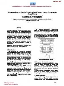
Discrete Wavelet Transform to Improve Guided-Wave-Based Health Monitoring of Tendons and Cables Piervincenzo Rizzo, Francesco Lanza di Scalea* NDE & Structural Health Monitoring (NDE/SHM) Laboratory Department of Structural Engineering, University of California, San Diego 9500 Gilman Drive, La Jolla, CA 92093-0085, USA

ABSTRACT Multi-wire steel strands are used in civil structures as pre-stressing tendons in prestressed concrete and as stay-cables in cable-stayed and suspension bridges. Monitoring the structural performance of these components is important to ensure the proper functioning and safety of the entire structure. Among the various NDE techniques that are under investigation for monitoring tendons and cables, the use of ultrasonic guided waves shows good promises. The main advantage of this approach is the possibility for the simultaneous monitoring of loads and detection of defects, such as corrosion and broken wires, by using the same ultrasonic setup. Load monitoring is achieved by measuring the travel time of the wave across a given length of the cable. Defect detection is achieved by measuring the reflections of the wave from the geometrical discontinuities. In this paper we present the enhancement on defect detection by implementing the Discrete Wavelet Transform (DWT) as a data post-processing tool. The data de-noising and data compression abilities of the DWT allow for greater sensitivity, larger ranges and higher monitoring speed. It is shown that the implementation of the DWT in the ultrasonic guided-wave technique becomes necessary for monitoring tendons and cables in the field.

1. INTRODUCTION Multi-wire steel strands are used as load-carrying members in civil structures like prestressed concrete structures and cablestayed and suspension bridges. The early and accurate detection of structural defects in these components is the subject of much current research in the Non-Destructive Evaluation (NDE) and structural health monitoring communities. Defects that can develop in the strands include corrosion, indentations and accidental fractured wires. Techniques based on ultrasonic stress waves have been under investigation for several years for the structural health monitoring of strands. Such techniques include the “active” method of Guided Ultrasonic Wave Testing (GUWT) and the “passive” method of Acoustic Emission Testing (AET). GUWT can potentially provide both load monitoring and defect detection capabilities. Several previous studies exist on the use of guided waves for the evaluation of stress levels in post-tensioning rods and multi-wire strands [1-4]. Defect detection in strands by GUWT was the topic of works at the SouthWest Research Institute [1,5,6] and at the Imperial College in London [7,8]. The inspection of the interface between steel bars and concrete in post-tensioned structures is another successful application of GUWT [9]. Passive AET has also been applied successfully to the real-time monitoring of evolving defects in both steel and composite cables [6,10,11,12]. One of the main advantages of guided-wave applications is the possibility of probing long length of the structure at once. A possible GUWT setup uses non-contact magnetostrictive sensors (MsS) to excite and detect the ultrasonic waves. MsS lend themselves to the inspection of cylindrical waveguides when access to the ends is not allowed and thus conventional piezoelectric transducers cannot be employed [1,3-6]. When compared to conventional “contact” piezoelectric transducers, the flexibility of MsS comes at the expense a reduced signal-to-noise ratio (SNR) of the ultrasonic measurements. This is generally the case with any “non-contact” ultrasonic transduction mechanism. Guided wave attenuation contributes to reducing the SNR of an ultrasonic defect signature. The situation is even more critical when the detection of small defects such as indentations is attempted. One effective tool that is gaining increasing attention to enhance the SNR of ultrasonic testing in real-time is a joint time-frequency analysis based on the Discrete Wavelet Transform (DWT). The two outcomes of a proper implementation of DWT processing are signal de-noising and signal compression [13,14].

*

Correspondence: Email: [email protected]; WWW: http://www.structures.ucsd.edu/; Phone: (858) 822-1458 Fax: (858) 534-6373

This paper demonstrates the de-noising capabilities of the DWT as applied to GUWT of strands. The dramatic improvement in SNR of the measurements can be utilized to effectively increase the inspection range and the defect detection sensitivity in the strands. Another useful outcome is the possibility of reducing the power supply to the transmitting probe. 2. THE DISCRETE WAVELET TRANSFORM

Wf(n,s) = N

-1/2

Wf(Nn,Ns)

3

(a)

Amplitude (V)

2 1 0 -1 -2

defect reflection

-3 3

Amplitude (V)

2.1 Theoretical background Wavelet transforms retain both the time and the frequency resolution overcoming the lose of time resolution of non-stationary signals, typical of the Fourier transforms. The wavelet transforms decompose the original signal by computing its correlation with a short-duration wave called the mother wavelet that is flexible in time and in frequency. For high-speed applications, the Discrete Wavelet Transform (DWT) implemented with parallel filter banks is a good choice because of its computational efficiency. The efficiency results from the existence of a fast orthogonal wavelet transform algorithm based on a set of filter banks [15-16]. The DWT may be intuitively considered as a decomposition of a function (signal) following hierarchical steps (levels) of different resolutions. At the first step the function is decomposed into wavelet coefficients; lowfrequency components (low-pass filtering) and high-frequency components (high-pass filtering) of the function are retained. The signal is therefore decomposed into separate frequency bands (scales). The filtering outputs are then downsampled. The number of wavelet coefficients for each branch is thus reduced by a factor of 2 such that the total number of points at a given level is that of the original signal. Each level j corresponds to a dyadic scale 2j at the resolution -j 2 . Furthering the decomposition means increasing the scale that corresponds to zooming into the low-frequency portions of the spectrum. Because of the downsampling, a signal of 2u points can be decomposed into u levels, which will u+1 sets of coefficients. produce a total of 2 Analytically, the wavelet transform of a time signal f(t) with N number of points can be described by the following equation

(b)

2 1 0 -1 -2 -3

35

65

95

125 155 185 Time (µsec)

 t  ⋅ψ  − n  j 2  2j

1

245

275

(c) D1

D2 D3

(1)

where n is the translation parameter and s is the scaling parameter. The parameter n shifts the wavelet in time and s controls the wavelet frequency bandwidth hence the time-frequency resolution of the analysis. The DWT of the j discrete signal f(t) is computed at scales s = 2 . Given a wavelet ψ(t), expressed as

ψ j , n (t ) =

215

(2)

the DWT of the function f(t) is calculated by the inner product

D4

D5

defect reflection

D6 35

95 155 215 275 Time (µsec)

35

95 155 215 275 Time (µsec)

Fig. 1. (a) Signal in seven-wire strand after 500 averages; (b) signal with no averages; (c) reconstructed signal after pruning the DWT coefficients at the first six decomposition levels.

+∞

W j , n = ∫ f (t ) ψ (t )*j , n dt

(3)

−∞

where ψ(t)* is the conjugate of ψ(t), and Wj,n are the detail coefficients. From the wavelet coefficients the initial function is reconstructed by the equation

f (t ) = ∑ ∑ W j ,nψ j n

j ,n

(4)

A complete review of the DWT algorithm is given Ref. [17]. 2.2 De-noising by pruning De-nosing and compression of the original signal can be achieved if only a few wavelet coefficients representative of the signal are retained and the remaining coefficients, related to noise, are discarded. This task is known as pruning [18]. The coefficients are upsampled to regain their original number of points and then passed through a reconstruction lowpass filters. The reconstruction filters are closely related but not equal to those of the decomposition tree. Reconstruction by using the k decomposition level k (scale 2 ), for example, is achieved by setting the wavelet coefficients from other scales equal to zero: Wj,n = 0 (j = 1,2,…,k-1, k+1,…,u)

(5)

Finally, the linear combination of the reconstructions from various decomposition levels results in the reconstruction of the original time signal. Figure 1 illustrates the pruning of an ultrasonic stress waves propagating in strands. Figure 1a shows a typical ultrasonic signal detected in a seven-wire, 15.24mm (0.6in)-diameter steel strand after 500 averages to reduce incoherent noise. The generation signal was a toneburst centered at 320 kHz. The acquisition sampling frequency was 33 MHz for all time signals shown in this paper. The signal detected at around 140 microseconds is the reflection from a 2.5mm-deep indentation in one of the helical wires of the strand. A single signal (no averages) is shown in Figure 1b where the defect reflection is completely buried in noise. The no-average signals reconstructed from the first six DWT decomposition levels are indicated in this figure as D1, D2,…, D6. The Daubechies wavelet of order 40 (db40) was used as the mother wavelet. Reconstruction D1 corresponds to what the time signal would look like if only level 1 highpass filter coefficient, cD1, were used for the reconstruction. D2 corresponds to what the reconstructed time signal would look like if only level 2 highpass filter coefficient, cD2, were used to reconstruct the signal, and so on. When choosing which filter levels should be selected to reconstruct the time signal, the criterion used was to select the filter level producing a synthetic time signal that most closely resembled the actual signal being analyzed. The result of averaging the raw ultrasonic measurements 500 times was the comparison signal. The filter associated with D6 in Figure 1c appears to yield the best reconstruction given the close resemblance with the averaged result in Figure 1a. Levels 1 to 5 will merely reconstruct noise. A thresholding step can be used after the pruning process to further increase the SNR [13]. In this case, a threshold is applied to the magnitude of the coefficients that are retained. This step assumes that the smaller coefficients represent noise, and can be safely omitted. Hence the data compression outcome of the DWT processing. It is important to emphasize that the success of a proper DWT decomposition is dependent on choosing a mother wavelet that best matches the shape of the signal that is being analyzed [18-19]. 3. STRAND INSPECTION SETUP Seven-wire strands with a diameter of 15.24 mm (0.6 in) were tested. MsS transducers were used for exciting and detecting ultrasonic guided waves in the strands. The distance between the transmitting sensor and the receiving sensor was fixed at 203 mm (8 in) in all tests. The sensors had a narrow frequency response centered at 320 kHz. The same sensors were successfully employed by the authors for stress measurement in similar strands using the acousto-elastic and elongation effects [4]. The choice of excitation frequency followed a broadband laser ultrasonic tests recently performed on strands under service loads where we examined the wave dispersion and attenuation at the level of the individual wires, namely the central, straight wire and the peripheral, helical wires. The study has addressed the role of applied load level on guided waves propagating in the strands and has shown that the first longitudinal mode propagates with reasonably little attenuation in the frequency range 300 kHz - 330 kHz [20]. In the present work, the test strands were subjected to a 120 kN tensile load corresponding to 45% of the material’s ultimate tensile strength (U.T.S.). The level represents a recommended service load for cable stays. Two different strands with artificially-created defects were tested. In the first specimen a sharp notch was machined in one of the helical wires by saw-cutting; different notch depths were monitored with varying notch-receiver distance. This test showed the effectiveness of the DWT-processed signals for the detection of small defects located away from the inspection sensors (long-range). In the second specimen two notches were cut in the top and bottom anchored regions of the strand. Each notch

was cut to a depth of 2.5 mm in two adjacent helical wires. The aim of this test was to probe the critical anchored areas that are subjected to stress concentrations and particularly prone to corrosion and other flaws in the field. © A National Instruments PXI unit running under LabVIEW was employed for signal excitation, detection and analysis. This unit was assembled and programmed at UCSD’s NDE & Structural Health Monitoring Laboratory for high-power, narrow-band ultrasonic testing applications. Five-cycle tonebursts centered at 320 kHz, modulated with a triangular window, were used as © generation signals. The DWT processing was done in real-time with the data acquisition in a MatLab environment linked to the main LabVIEW program.

Unprocessed data: no averages

Unprocessed data: 500 averages

1 0 -1 -2

1 0 -1

Amplitude (V)

Amplitude (V)

2

Amplitude (V)

2 1 0 -1 -2 460 500 540 580 620 660 700 Time (µsec)

Amplitude (V)

-2

Amplitude (V)

-.5

.5

-.5 -1

1

1

.5 0 -.5

.5

-.5 -1

1

1

0 -.5

.5

-.5 -1

1

1

0 -.5 -1

3.0 mm notch depth

0

-1

.5

1.5 mm notch depth

0

-1

.5

No defect

0

-1

Amplitude (V)

2

Amplitude (V)

Amplitude (V)

3

0

Amplitude (V)

-2

.5

Amplitude (V)

-1

Amplitude (V)

Amplitude (V)

0

1

1

2 1

Reconstructed D6: no averages

.5

Broken wire

0 -.5 -1

460 500 540 580 620 660 700 Time (µsec)

= defect reflection

460 500 540 580 620 660 700 Time (µsec)

= end reflection

Fig. 2. Signals in strand with no averages (left column), after 500 averages (middle column), and after D6 reconstruction with db40 wavelet (right column).

4. RESULTS 4.1 Role of the mother wavelet As mentioned above, the selection of a proper mother wavelet is determinant for a successful application of the DWT algorithm. The similarity between the shape of the mother wavelet and the shape of the expected signal is the guideline for the choice of a proper wavelet. A signal obtained with an elevated number of averages can be considered a good target when the SNR of a single event is too low. This is the case of a reflection from a small defect located far away from the inspection probes. It was shown [20] that for this application the level D6 reconstruction (pruning) of the db40 yields a better reconstruction of the signal. By comparing the db40 and the reconstruction form the coiflet mother wavelet of the first order (coif1), it was shown that coif 1 alters alters the shape of the signal in the time domain, and, in the frequency domain, underestimates the center peak amplitude and it produces spurious peaks.

Reflection Coefficient

4.2 Defect detection: free strands The db40 with a D6 reconstruction was used in the DWT signal processing for the strand specimens. In the first specimen the notch was machined in a helical wire with depths increasing by 0.5 mm to a maximum depth of 3 mm. A final cut resulted in the complete fracture of the helical wire, which was the largest defect examined in this specimen. It should be pointed out that the geometry of the saw was such that cutting the individual wire at depths of 2.5 mm and 3 mm also produced small indentation in the two adjacent wires. Reflected signals from the defect were collected with varying notchreceiver distances from a minimum of 203 mm (8 in) to a maximum of 1,118 mm (44 in) that was the largest distance allowed by the loading frame. Representative results are presented in Figure 2. The cases of no defect, 1.5mm0.8 deep notch, 3mm-deep notch and broken wire are shown in * Unprocessed data this figure. The results were Reconstructed D6 obtained with the largest 1 2 5 10 50 500 0.6 notch-receiver distance of 1,118 mm. In all plots the later signal is the reflection from the strand flat end that is detected at around 620 µsec. 0.4 The left column presents the unprocessed signals detected in a single generation event (no averages). The middle 1 2 5 10 50 500 0.2 column presents the unprocessed signals 1 2 5 10 50 500 averaged 500 times. The 1 2 5 10 50 500 DWT-processed signals are 1 2 5 10 50 500 0 shown in the right column with no averages taken. The 1.5 mm 2.0 mm 2.5 mm 3.0 mm broken wire benefit of using DWT processing for the detection of Notch Depth the defect reflection, occurring Fig. 3. Reflection coefficients from notches of varying depths as a function of number of at around 540 µsec, can be averages (from 1 to 500) without wavelet processing and with wavelet processing. clearly seen. DWT processing dramatically increases the sensitivity to the defect signatures. The results in Figure 2 show that the DWT processing performed with an appropriate mother wavelet and pruning procedure de-noises the signals with at least the same effectiveness as averaging 500 times. In order to further emphasize the effectiveness and robustness of the DWT processing, the ultrasonic Reflection Coefficients from the notches were calculated and compared to those obtained by averaging without DWT processing. Reflection coefficients were calculated by normalizing the amplitude of the defect reflection with that of the first arrival at the receiving probe (incoming signal). Figure 3 summarizes the results for the notch depths of 1.5 mm, 2 mm, 2.5 mm and 3 mm, along with the broken wire case. The DWT results are more stable than the unprocessed results that are highly dependent on the number of signal averages used. A few missing data for the unprocessed case reflect the poor SNR of the defect signatures at small number of averages. Also, some of the unprocessed data yield unrealistically large reflection coefficients. On the contrary, the DWT processing results into more stable results in all cases, including the small defect cases, without the necessity for averaging. In addition, it can be seen that the reflection coefficients from the DWT processing are generally larger than those obtained without processing. This beneficial effect results from the larger SNR of the defect reflections, since noise is not an issue for the incoming signals (the shortest transmitter-receiver path).

1.5

direct-path signal

Amplitude (V)

1.0

(a)

end reflection (a)

0.5 0 -0.5 -1.0

defect

-1.5 1.5 (b)

Amplitude (V)

1.0 0.5 0 -0.5 -1.0

defect

-1.5 0.45 (c)

0.30

Amplitude (V)

With the second strand specimen the aim was to probe the notches machined in the anchored regions as a critical portion of the strand. The presence of the anchorages reduces the ultrasonic energy of the propagating wave due to to leakage into the adjacent wedges. The acoustic leakage from the strand into the anchorage blocks was exploited to monitor conveniently ongoing damage in the strands by acoustic emission testing [16]. In the context of the present investigation, acoustic leakage makes the detection of notches more challenging by further reducing the SNR of the measurements. Representative results are shown in Figure 4. The unprocessed time waveform (1000 averages) is presented in Figure 4a. The first signal is the direct wave traveling from the MsS transmitter to the MsS receiver. The reflection from the strand free end is seen arriving at around 200 µsec. Shortly earlier, at around 175 µsec, the reflection from the defect can be seen (2.5mm-deep notches in two adjacent helical wires in the anchored area). The DWT-processed signal with no averages (D6 reconstruction) is presented in Figure 4b. The similarity with Figure 4a is evident showing, again, that the processing virtually eliminates the need for averaging. The results in Figure 4b were obtained by using a high-power toneburst signal driving the MsS transmitter with a 150V peak-to-peak magnitude. The high power helps increasing the sensitivity to the defect by partially compensating for the acoustic losses in the anchorage block. Increasing the generation power is routinely done in inspections of highly attenuating components. Unfortunately, a low-power inspection system is obviously desirable in a field application. Figure 4c shows the DWT-processed signal (no averages) detected by lowering the generation signal to a 10V p-p toneburst. This represents a 15-fold amplitude decrease from the previous case. The energy of the detected signals is reduced accordingly (note the different ordinate scale in Figure 4c). Nevertheless, the defect signature is still detected at around 175 µsec.

0.15 0

-0.15 -0.30

defect reflection

-0.45 35

75

115

155

195

235

275

Time (µsec) Fig. 4. (a) Signals detected through the anchored region of the strand after 1000 averages; (b) after wavelet processing with a 150V p-p generation toneburst to the transmitting probe; (c) after wavelet processing with a 10V p-p generation toneburst.

4.3 Defect detection: embedded strands The detection of the defects in embedded steel strands is discussed here. The idea we propose aim at developing an array of magnetostrictive sensors that can be embedded with the strand for the active inspection of prestressed structures. The application is dedicated to the going to be built structures and cannot be applied to existing structures. First attempt is dedicated to the simple case of a stress-free strand of 0.6 inches diameter, enclosed in a plastic pipe, 63.5 mm (2.5 inches) diameter filled with commercial grout. The strand examined was 1538 mm long. Two notches were artificially created by saw-cutting machine. Notch N1 consisted of two peripheral wires cut at half of their diameter; the second notch (N2) consist of three peripheral wires cut with one of them completely broken. Three MsS were employed, one transmitter (T) and two receivers (RA and RB). The transmitter was placed in a symmetrical position respect to the receivers. Notch (N1) was machined between the transmitter and the receiver RB, whereas the other notch was between the receiver RA and the right end of the strand. To avoid that grout does fill the notches a thin layer of adhesive tape was used to cover the notch areas. The plastic pipe was 1400 mm long, which therefore represent the length of the grouted segment. Figure 5 schematizes the setup.

RB

400

Notch N1

308

T

152 310 1400 (grouted portion)

RA

Notch N2

208

197 51

1538 Fig. 5. Defect detection in a stress-free grouted strand. Schematic setup. Distances expressed in mm.

Amplitude (mV)

Amplitude (mV)

For this purpose, sensors resonant at 380 kHz were used. A PXI unit connected with a RITEC-2500 gated amplifier was used. The RITEC boosted the toneburst coming from the PXI up to 50 Volts peak-to peak. Five cycles, 380 kHz windowed toneburst was generated. The received signal was amplified with a pre-amp set at 60 dB, averaged 800 times and stored with 10 MHz sampling frequency. Here, we present the results of a test performed 24 hours after pouring the grout inside the pipe (Figure 6). The reconstructed D4 signal of the waves detected with receiver A is plotted in Figure 6a. The mother wavelet db40 was used. The big initial signal is due to the electromagnetic spike. More important at almost 50 microseconds the direct signal traveling from the transmitter to the receiver is clearly detected. Beyond this other perturbations are detected. Centered at around 132 microseconds and at 155 microseconds are detected the signals coming from the reflection with notch N1 and N2, respectively. Signals have covered a path length equal to 614 mm and 726 mm, respectively. In addition the reflection from 80 the right end side, expected at around 260 microseconds is visible. Despite the perturbation (a) 60 crosses notch 1 twice, the wave is detected. The reconstructed D4 signal for signal detected with 40 receiver B is plotted in Figure 6b. Direct signal from transmitter to receiver B is detected at 50 microseconds. Echo from right end 20 Signal peak amplitude is halved compared to Figure 6a. The wave traveling from transmitter to sensor B 0 encounters the notch N1 that reduces the acoustic energy (lower peak amplitude) and scatters the signal -20 (slight larger duration). At around 260 kHz appears a Echo from N2: T→ N2→RA signal due to the combination of the wave reflection from -40 left end and from notch N2. Those signals have traveled Echo from N1: T→ N1→RA 1448 mm and 1496 mm (almost 5 feet), respectively. -60 Direct signal: T→RA CONCLUSIONS -80 Signal processing based on the Discrete Wavelet Transform (DWT) was employed to enhance ultrasonic 80 health monitoring of seven-wire steel strands. (b) Magnetostrictive sensors for the excitation and the 60 detection of guided waves in the strands were used. The non-contact character of these sensors, coupled 40 Combination of left end with the necessity for detecting small defects at large reflection and echo from N2 distances (long-range inspection), motivate the need for 20 enhancing the sensitivity of the defect detection procedure. The unmatched de-noising performance of 0 the DWT was exploited to increase the SNR of the measurements in real time while reducing, if not -20 eliminating, the need for signal averaging. The Daubechies wavelet of order 40 was shown to be -40 effective for the subject application due to its narrowband character resembling that of the generation Direct signal: T→RA -60 toneburst. Effective de-noising was demonstrated by pruning the DWT filter bank decomposition of the -80 reflections from sharp notches as shallow as 1.5 mm 0 45 90 135 180 225 270 315 360 405 450 and as far away as 1.1 m (44 in) from the receiving probe. In this case, the DWT processing of a single Time (µsec) signal was shown to be at least as effective for defect Fig. 6. Defect detection in a stress-free grouted strand. detection as performing 500 averages. The processing Reconstructed D4 signal from (a) sensor RA and from (b) sensor Rb.

proved particularly robust when reflection coefficients from the defects were obtained. Notches located in the anchored regions of the strand were also examined. In this case, DWT processing was as effective as performing 1,000 averages in detecting two, 2.5mm-deep notches. The wavelet processing allowed for the use a low-power source, rather than a highpower one. Low power is highly desirable for any field monitoring. In particular, it was shown that a 10 V peak-to-peak generation signal can be as effective as a 150 V peak-to-peak signal in detecting the notches in the anchored areas once DWT processing is used. Finally, the pilot results from an innovative employment of MsS for the generation and detection of ultrasonic waves in grouted strands is shown. In summary, the DWT emerges as a powerful tool to ease the transition to the field of guided-wave ultrasonic monitoring of strands. ACKNOWLEDGMENTS This work was supported by the National Science Foundation grant CMS-0221707 (S-C. Liu, Program Director) and by the 2002 American Society for Non-Destructive Testing (ASNT) Research Fellowship Award. REFERENCES 1. Kwun, H., Bartels, K. A. and Hanley, J. J., “Effect of tensile loading on the properties of elastic-wave propagation in a strand,” J. Acoust. Soc. Am., 103, 3370-3375, 1998. 2. Chen, H-L. and Wissawapaisal, K., “Application of Wigner-Ville transform to evaluate tensile forces in seven-wire prestressing strands,” ASCE J. Eng. Mech., 128, 1206-1214, 2002. 3. Washer, G. A., Green, R. E., and Pond, R. B., “Velocity constants for ultrasonic stress measurements in prestressing tendons,” Res. Nondestr. Eval., 14, 81-94, 2002. 4. Lanza di Scalea, F., Rizzo, P. and Seible, F., “Stress measurement and defect detection in steel strands by guided stress waves,” ASCE J. Mat. in Civ. Eng., 15, 219-227, 2003 5. Kwun, H. and Teller, C. M., “Detection of fractured wires in steel cables using magnetostrictive sensors,” Mater. Eval., 52, 503-507, 1994 6. Kwun, H. and Teller, C. M., “Nondestructive evaluation of steel cables and ropes using magnetostrictively induced ultrasonic waves and magnetostrictively detected acoustic emissions,” U.S. Patent No. 5,456,113, 1995. 7. Pavlakovic, B. N., Lowe, M. J. S. and Cawley, P., “The inspection of tendons in post-tensioned concrete using guided ultrasonic waves,” Insight, 41, 446-452, 1999. 8. Beard, M. D., Lowe, M. J. S. and Cawley, P., “Ultrasonic guided waves for inspection of grouted tendons and bolts,” ASCE J. Mat. in Civ. Eng., 15, 212-218, 2003. 9. Na, W-B. and Kundu, T., “A Combination of PZT and EMAT transducers for interface inspection,” J. Acoust. Soc. Am., 111, 2128-2139, 2002. 10. Laura, P. A. A., Vanderveldt, H. and Gaffney, P. G., “Acoustic detection of structural failure of mechanical cables,” J. Acoust. Soc. Am., 45, 791-793, 1969. 11. Casey, N. F. and Laura, P. A. A., “A review of the acoustic-emission monitoring of wire ropes,” Ocean Engng., 24, 935947, 1997. 12. Rizzo, P. and Lanza di Scalea, F., “Acoustic emission monitoring of carbon-fiber-reinforced-polymer bridge stay cables in large-scale testing,” Exp. Mech., 41, 282-290, 2001. 13. Abbate, A., Koay, J., Frankel, J., Schroeder, S. C. and Das, P., “Signal detection and noise suppression using a wavelet transform signal processor: application to ultrasonic flaw Detection,” IEEE UFFC, 44, 14-26, 1997. 14. Legendre, S., Massicotte, D., Goyette, J. and Bose, T. K., “Wavelet-transform-based method of analysis for Lamb-wave ultrasonic NDE signals,” IEEE Trans. Instrumentation and Measurement, 49, 524-530, 2000. 15. Mallat S. G., “A theory for multiresolution signal decomposition: the wavelet representation,” IEEE Trans. Pattern Analysis and Machine Intelligence, 11, 674-693, 1989. 16. Mallat, S. G., A Wavelet Tour of Signal Processing, Academic Press, New York, 1999. 17. Rizzo, P. and Lanza di Scalea, F., “Ultrasonic Inspection of Multi-Wire Steel Strands With the Aid of the Wavelet Transform”, submitted for publication. 18. Petropulu, A, “Detection of transients using discrete wavelet transform,” ICASSP-92: IEEE Int. Conf. Acoust. Speech, Signal Processing, 2, 477-480, 1992. 19. Abbate, A., Koay J., Frankel, J., Schroeder, S. C. and Das, P., “Application of wavelet transform signal processor to ultrasound,” Proc. 1994 Ultrasonic Symposium, 94CH3468-6, 1147-1152, 1994. 20. Rizzo, P. and Lanza di Scalea, F., “Dispersive wave propagation in multi-wire strands by laser ultrasound and wavelet transform,” Exp. Mech., in press.