DISTANCE-BASED INDEXING FOR HIGH-DIMENSIONAL METRIC SPACES*
Tolga Bozkaya
Meral Ozsoyoglu
Department of Computer Engineering & Science Case Western Reserve University email:
[email protected]
Department of Computer Engineering & Science Case Western Reserve University
[email protected]
Abstract In many database applications, one of the common queries is to find approximate matches to a given query item from a collection of data items. For example, given an image database, one may want to retrieve all images that are similar to a given query image. Distance based index structures are proposed for applications where the data domain is high dimensional, or the distance function used to compute distances between data objects is non-Euclidean. In this paper, we introduce a distance based index structure called multi-vantage point (mvp) tree for similarity queries on high-dimensional metric spaces. The mvptree uses more than one vantage point to partition the space into spherical cuts at each level. It also utilizes the pre-computed (at construction time) distances between the data points and the vantage points. We have done experiments to compare mvp-trees with vp-trees which have a similar partitioning strategy, but use only one vantage point at each level, and do not make use of the pre-computed distances. Empirical studies show that mvptree outperforms the vp-tree 20% to 80% for varying query ranges and different distance distributions. 1. Introduction In many database applications, it is desirable to be able to answer queries based on proximity such as asking for data items that are similar to a query item, or that are closest to a query item. We face such queries in the context of many database applications such as genetics, image/picture databases, time series analysis, information retrieval, etc. In genetics, the concern is to find DNA or protein sequences that are similar in a genetic database. In time-series analysis, we would like to find similar patterns among a given collection of sequences. Image databases can be queried to find and retrieve images in the database that are similar to the query image with respect to a specified criteria. * This research is partially supported by the National Science Foundation grant IRI 92-24660, and the National Science Foundation FAW award IRI90-24152
Similarity between images can be measured in a number of ways. Features such as shape, color, texture can be extracted from images in the database to be used as content information where the distance calculations will be based on. Images can also be compared on a pixel by pixel basis by calculating the distance between two images as the accumulation of the differences between the intensities of their pixels. In all the applications above, the problem is to find similar data items to a given query item where the similarity between items is computed by some distance function defined on the application domain. Our objective is to provide an efficient access mechanism to answer these similarity queries. In this paper, we consider the applications where the data domain is high dimensional, and the distance function employed is metric. It is important for an application to have a metric distance function to make it possible to do filtering of distant data items for a similarity query by using the triangle inequality property (section 2). Because of the high dimensionality, the distance calculations between data items are assumed to be very expensive. Therefore, an efficient access mechanism should certainly have to minimize the number of distance calculations for similarity queries to improve the speed in answering them. This is usually done by employing techniques and index structures that are used to filter out distant (non-similar) data items quickly, avoiding expensive distance computations for each of them. The data items that are in the result of a similarity query can be further filtered out by the user through visual browsing. This happens in image database applications where the user would pick the most semantically related images to a query image by examining the images retrieved as the result of a similarity query. This is mostly inevitable because it is impossible to extract and represent all the semantic information for an image simply by extracting features in the image. The best an image database can do is to present the images that are related or close to the query image, and leave the further identification and semantic interpretation of images to users. In this paper, we introduce the mvp-tree (multi-vantage point tree) as a general solution to the problem of answering similarity based queries efficiently for high-dimensional metric spaces. The mvp-tree is similar to the vp-tree (vantage point tree) [Uhl91] in the sense that both structures use relative distances from a vantage point to partition the domain space. In vp-trees, at every node of the tree, a vantage point is chosen among the data
points, and the distances of this vantage point from all other points (the points that will be indexed below that node) are computed. Then, these points are sorted into an ordered list with respect to their distances from the vantage point. Next, the list is partitioned at positions to create sublists of equal cardinality. The order of the tree corresponds to the number of partitions to be made. Each of these partitions keep the data points that fall into a spherical cut with inner and outer radii being the minimum and the maximum distances of these points from the vantage point. The mvp-tree behaves more cleverly in making use of the vantage-points by employing more than one at each level of the tree to increase the fanout of each node of the tree. In vp-trees, for a given similarity query, most of the distance computations made are between the query point and the vantage points. Because of using more than one vantage points in a node, the mvp-tree has less vantage points compared to a vp-tree. The distances of data points at the leaf nodes from the vantage points at higher levels (which were already computed at construction time) are kept in mvp-trees, and these distances are used for efficient filtering at search time. The efficient filtering at the leaf level is utilized more by making the leaf nodes to have higher node capacities. By this way, the major filtering step during search is delayed to the leaf level. We have done experiments with 20-dimensional Euclidean vectors and gray-level images to compare vp-trees and mvp-trees to demonstrate mvp-trees’ efficiency. The distance distribution of data points plays an important role in the efficiency of the index structures, so we experimented on two sets of Euclidean vectors with different distance distributions. In both cases, mvp-trees made 20% to 80% less number of distance computations compared to vp-trees for small query ranges. For higher query ranges, the percentagewise difference decreased gradually, yet the mvp-trees performed 10% to a respectable 30% less distance computations for the largest query ranges we used in our experiments. Our experiments on gray-level images using L1 and L2 metrics (see section 5.1) also revealed the fact that mvp-trees perform better than vp-trees. For this data set, we had only 1151 images to experiment on (and therefore had rather shallow trees), and the mvp-trees performed upto 20-30% less distance computations. The rest of the paper is organized as follows. Section 2 gives the definitions for high dimensional metric spaces and similarity queries. Section 3 presents the problem of indexing in high dimensional spaces and also presents previous approaches to this problem. The related work for distance-based index structures to answer similarity based queries is also given in section 3. Section 4 introduces the mvp-tree structure. The experimental results for comparing the mvp-trees with vp-trees are given in section 5. We summarize our results and point out future research directions in section 6. 2. Metric Spaces and Similarity Queries In this section, we briefly give the definitions for metric distance functions and different types of similarity queries.
A metric distance function d(x,y) for a metric space is defined as follows: i) d(x,y) = d(y,x) ii) 0 < d(x,y) < ∞, x≠ y iii) d(x,x) = 0 iv) d(x,y) ≤ d(x,z) + d(z,y)
(triangle inequality)
The above conditions are the only ones we should be assuming when designing an index structure based on distances between objects in a metric space. Note that, we cannot make use of any geometric information about the metric space, unlike the way we can for a Euclidean space. We only have a set of objects from a metric space, and a distance function d() that can be used to compute the distance between any two objects. Similarity based queries can be posed in a number of ways. The most common one asks for all data objects that are within some specified distance from a given query object. These queries require retrieval of near neighbors of the query object: Near Neighbor Query: From a given set of data objects X = {X1, X2, ..., Xn} from a metric space with a metric distance function d(), retrieve all data objects that are within distance r of a given query point Y. The resulting set will be { Xi | Xi ∈ X and d(Xi,Y)≤ r }. Here, r is generally referred to as the similarity measure, or the tolerance factor. Some variations of the near neighbor query are also possible. The nearest neighbor query asks for the closest object to a given query object. Similarly, k closest objects may be requested as well. Though not very common, objects that are farther than a given range from a query object can also be asked as well as the farthest, or the k farthest objects from the query object. The formulation of all these queries are similar to the near neighbor query we have given above. Here, we are mainly concerned on distance based indexing for high-dimensional metric spaces. We also concentrate on the near neighbor queries when we introduce our index structure. Our main objective is to minimize the number of distance calculations for a given similarity query as we assume that distance computations in high-dimensional metric spaces are very expensive. In the next section, we discuss the indexing problem for high-dimensional metric spaces, and review previous approaches to the problem. 3. Indexing in High-Dimensional Spaces For low-dimensional Euclidean domains, the conventional index structures ([Sam89]) such as R-trees (and its variations) [Gut84, SRF87, BKSS90] can be used effectively to answer similarity queries. In such cases, a near neighbor search query would ask for all the objects in (or that intersects) a spherical search window where the center is the query object and the radius is the tolerance factor r. There are some special techniques for other forms of similarity queries, such as nearest neighbor queries. For example, in [RKV95], some heuristics are introduced to efficiently search the R-tree structure to answer nearest neighbor queries. However, the conventional spatial structures stop being efficient if the dimensionality is high. Experimental results [Ott92] show that R-trees become inefficient for n-dimensional spaces where n is greater than 20.
The problem of indexing high-dimensional spaces can be approached in different ways. One approach is to use distance preserving transformations to Euclidean spaces, which we discuss in section 3.1. Another approach is using distance-based index structures. In section 3.2, we discuss distance-based index structures, and briefly review the previous work. In section 3.3, we discuss the vp-tree structure in detail since it is the most relevant approach to work. 3.1 Distance Preserving Transformations
domains as the conventional distance functions (such as Euclidean, or any Lp distance) used for these domains are metric. Sequence matching, time-series analysis, image databases are some example applications having such domains. Distance based techniques are also applicable for domains where the data is nonspatial (that is, data objects can not be mapped to points in a multi-dimensional space), such as in the case of text databases which generally use the edit distance (which is metric) for computing similarity data items (lines of text, words, etc.). We review a few of the distance based indexing techniques below.
There are ways to use conventional spatial structures for high-dimensional domains. One way is to apply a mapping of objects from a high-dimensional space to a low-dimensional (Euclidean) space by using a distance preserving transformation, and then using conventional index structures (such as R-trees) as a major filtering mechanism. A distance preserving transformation is a mapping from a high-dimensional domain to a lower-dimensional domain where the distances between objects before the transformation (in the actual space) are greater than or equal to the distances after the transformation (in the transformed space). That is, the distance preserving functions underestimate the actual distances between objects in the transformed space. Distance preserving transformations have been successfully used to index high-dimensional data in many applications such as time sequences [AFA93, FRM94], and images [FEF+94].
3.2 Distance-Based Index Structures
The distance preserving functions such as DFT, Karhunen-Loeve are applicable to any Euclidean domain. Yet, it is also possible to come up with application specific distance preserving transformations for the same purpose. In the QBIC (Query By Image Content) system [FEF+94], color content of images can be used to answer similarity queries. The difference of the color contents of two images are computed from their color histograms. Computation of a distance between the color histograms of two images is quite expensive as the color histograms are high-dimensional (number of different colors is generally 64 or 256) vectors, and also crosstalk (as some colors are similar) between colors have to be considered. To increase speed in color distance computation, the QBIC keeps an index on average color of images. The average color of an image is a 3dimensional vector with the average red, blue, and green values of the pixels in the image. The distance between average color vectors of images are proven to be less than or equal to the distance between their color histograms, that is, the transformation is distance preserving. Similarity queries on color content of images are answered by first using the index on average color vectors as the major filtering step, and then refining the result by actual computations of histogram distances.
In the second approach in [BK73], they partition the space into a number of sets of keys. For each set, they arbitrarily pick a center key, and calculate the radius which is the maximum distance between the center and any other key in the set. The keys in a set are partitioned into other sets recursively creating a multi-way tree. Each node in the tree, keeps the centers and the radii for the sets of keys indexed below. The strategy for partitioning the keys into sets was not discussed and was left as a parameter.
Note that, although the idea of using distance preserving transformation works fine for many applications, it makes the assumption that such a transformation exists and applicable to the application domain. Transformations such as DFT or Karhunen-Loeve are not effective in indexing high-dimensional vectors where the values at each dimension are uncorrelated for any given vector. Therefore, unfortunately, it is not always possible or cost effective to employ this method. Yet, there are distance based indexing techniques that are applicable to all domains where metric distance functions are employed. These techniques can be directly employed for high-dimensional spatial
There are a number of research results on efficiently answering similarity search queries in different contexts. In [BK73], Burkhard & Keller suggested the use of three different techniques for the problem of finding best matching (closest) key words in a file to a given query key. They employ a metric distance function on the key space which always returns discrete values, (i.e., the distances are always integers). Their first method is a hierarchical multi-way tree decomposition. At the top level, they pick an arbitrary element from the key domain, and group the rest of the keys with respect to their distances to that key. The keys that are of the same distance from that key get into the same group. Note that this is possible since the distance values are always discrete. The same hierarchical composition goes on for all the groups recursively, creating a tree structure.
The third approach of [BK73] is similar to the second one, but there is the requirement that the diameter (the maximum distance between any two points in a group) of any group should be less than a given constant k, where the value of k is different at each level. The group satisfying this criterion is called a clique. This method relies on finding the set of maximal cliques at each level, and keeping their representatives in the nodes to direct or trim the search. Note that keys may appear in more than one clique, so the aim is to select the representative keys to be the ones that appear in as many cliques as possible. In another approach, such as the one in [SW90], precomputed distances between the data elements are used to efficiently answer similarity search queries. The aim is to minimize the number of distance computations as much as possible, as they are assumed to be very expensive. Search algorithms of O(n) or even O(n log n) (where n is the number of data objects) are acceptable if they minimize the number distance computations. In [SW90], a table of size O(n2) keeps the distances between data objects if they are pre-computed. The other pairwise distances are estimated (by specifying an interval) by making use of the other pre-computed distances. The technique of storing and using pre-computed distances may be effective for data domains with small cardinality, however, the
space requirements and the search complexity becomes overwhelming for larger domains. In [Uhl91], Uhlmann introduced two hierarchical index structures for similarity search. The first one is the vp-tree (vantage-point tree). The vp-tree basically partitions the data space into spherical cuts around a chosen vantage point at each level. This approach, referred to as the ball decomposition in the paper is similar to the first method presented in [BK73]. At each node, the distances between the vantage point for that node and the data points to be indexed below that node are computed. The median is found, and the data points are partitioned into two groups, one of them accommodating the points whose distances to the vantage point are less than or equal to the median distance, and the other group accommodating the points whose distances are larger than or equal to the median. These two groups of data points are indexed separately by the left and right subbranches below that node, which are constructed in the same way recursively. Although the vp-tree was introduced as a binary tree, it is also possible to generalize it to a multi-way tree for larger fanouts. In [Yia93], the vp-tree structure was enhanced by an algorithm to pick vantage-points for better decompositions. In [Chi94] the vp-tree structure is modified to answer nearest neighbor queries. We talk about the vp-trees in detail in section 3.3. The gh-tree (generalized hyperplane tree) structure was also introduced in [Uhl91]. It is constructed as follows. At the top node, two points are picked and the remaining points are divided into two groups depending on which of these two points they are closer to. The two branches for the two groups are built recursively in the same way. Unlike the vp-trees, the branching factor can only be two. If the two pivot points are well-selected at every level, the gh-tree tends to be a well-balanced structure. More recently, Brin introduced the GNAT (Geometric Near-Neighbor Access Tree) structure [Bri95]. A k number of split points are chosen at the top level. Each one of the remaining points are associated with one of the k datasets (one for each split point), depending on which split point they are closest to. For each split point, the minimum and maximum distances from the points in the datasets of other split points are recorded. The tree is recursively built for each dataset at the next level. The number of split points, k, is parameterized and is chosen to be a different value for each data set depending on its cardinality. The GNAT structure is compared to the binary vp-tree, and it is shown that the preprocessing (construction) step of GNAT is more expensive than the vp-tree, but its search algorithm makes less number of distance computations in the experiments for different data sets. 3.3 Vantage point tree structure Let us briefly discuss the vp-trees to explain the idea of partitioning the data space around selected points (vantage points) at different levels forming a hierarchical tree structure and using it for effective filtering in similarity search queries. The structure of a binary vp-tree is very simple. Each internal node is of the form (Sv, M, Rptr, Lptr), where Sv is the vantage point, M is the median distance among the distances of
all the points (from Sv) indexed below that node, and Rptr and Lptr are pointers to the right and left branches. Left branch of the node indexes the points whose distances from Sv are less than or equal to M, and right branch of the node indexes the points whose distances from Sv are greater than or equal to M. In leaf nodes, instead of the pointers to the left and right branches, references to the data points are kept. Given a finite set S={S1, S2, .. , Sn} of n objects, and a metric distance function d(Si, Sj), a binary vp-tree V on S is constructed as follows. 1) If S= 0, then create an empty tree. 2) Else, let Sv be an arbitrary object from S. (Sv is the vantage point) M = median of { d(Si, Sv) | ∀Si ∈ S} Let Sl = { Si | d(Si, Sv) ≤ M, where Si ∈ S and Si ≠ Sv} Sr = { Sj | d(Sj, Sv) ≥ M, where Sj ∈ S} (the cardinality of Sl and Sr should be equal) Recursively create vp-trees on Sl and on Sr as the left and right branches of the root of V. The binary vp-tree is balanced and therefore can be easily paged for storage in secondary memory. The construction step requires O(n log2 n) distance computations. For a given query object Q, the set of data objects that are within distance r of Q are found using the search algorithm given below. 1) If d(Q , Sv) ≤ r, then Sv (the vantage point at the root) is in the answer set. 2) If d(Q, Sv) + r ≥ M (median), then recursively search the right branch 3) If d(Q, Sv) - r ≤ M, then recursively search the left branch. (note that both branches can be searched if both search conditions are satisfied) The correctness of this simple search strategy can be proven easily by using the triangle inequality of distances among any three objects in a metric data space (see Appendix). Generalizing binary vp-trees into multi-way vp-trees. The binary vp-tree can be easily generalized into a multiway tree structure for larger fanouts at every node hoping that the decrease in the height of the tree would also decrease the number of distance computations. The construction of a vp-tree of order m is very similar to that of a binary vp-tree. Here, instead of finding the median of the distances between the vantage point and the data points, the points are ordered with respect to their distances from the vantage point, and partitioned into m groups of equal cardinality. The distance values used to partition the data points are recorded in each node. We will refer to those values as cutoff values. There are m-1 cutoff values in a node. The m groups of data points are indexed below the root node by its m children, which are themselves vp-trees of order m created in the same way recursively. The construction of an m-way vptree requires O(n log m n) distance computations. That is, creating an m-way vp-tree decreases the number of distance computations by a factor of log2 m compared to binary vp-trees at the construction stage.
3
leaf nodes for effective filtering of non qualifying points in a similarity search operation. 4.1 Motivation
2 1 R1
R2
Figure 1. The root level partitioning of a vp-tree with branching factor 3. The three different regions are labelled 1, 2, 3, and they are all shaded differently.
However, there is one problem with high-order vp-trees when the order is large. The vp-tree partitions the data space into spherical cuts (see Figure 1). Those spherical cuts become too thin for high-dimensional domains, leading the search regions to intersect with many of them, and therefore leading to more branching in doing similarity searches. As an example, consider an N-dimensional Euclidean Space where N is a large number, and a vp-tree of order 3 is built to index the uniformly distributed data points in that space. At the root level, the N-dimensional space is partitioned into three spherical regions, as shown in Figure 1. The three different regions are colored differently and labeled as 1, 2, and 3. Let R1 be the radius of region 1, and R2 be the radius of the sphere enclosing regions 1 and 2. Because of the uniform distribution assumption, we can consider the Ndimensional volumes of regions 1 and 2 to be equal. The volume of an N-dimensional sphere is directly proportional to the Nth factor of its radius, so we can deduce that R2 = R1 * (2)1/N . The thickness of the spherical shell of region 2 is R2 - R1 = R1 *( 21/N - 1). To give an idea, for N=100, R2 = 1.007 R1. So, when the spherical cuts are very thin, the chances of a search operation descending down to more than one branch becomes higher. If a search path descends down to k out of m children of a node, then k distance computations are needed at the next level, where the distance between the query point and the vantage point of each child node has to be found. This is because the vp-tree keeps a different vantage point for each node at the same level. Each child of a node is associated with a region that is like a spherical shell (other than the innermost child, which has a spherical region), and the data points indexed below that child node all belong to that region. Those regions are disjoint for the siblings. As the vantage point for a node has to be chosen among the data points indexed below a node, the vantage points of the siblings are all different. 4. Multi-vantage-point trees In this section, we present the mvp-tree (multi vantage point tree). Similar to the vp-tree, the mvp-tree partitions the data space into spherical cuts around vantage points. However, it creates partitions with respect to more than one vantage point at one level and keeps extra information for the data points in the
Before we introduce the mvp-tree, we first discuss a few useful observations that can be used as heuristics for a better search structure. The idea is to partition the data space around a vantage point at each level for a hierarchical search. Observation 1: It is possible to partition a spherical shell-like region using a vantage point chosen from outside the region. This is shown in Figure 2, where a vantage point outside of the region is used to partition it into three parts, which are labeled as 1,2,3 and shaded differently (region 2 consists of two disjoint parts). The vantage point does not have to be from inside the region, unlike the strategy followed in vp-trees.
Figure 2. Partitioning a spherical shell-like region using a vantage point from outside. This means that we can use the same vantage point to partition the regions associated with the nodes at the same level. When the search operation descends down to several branches, we do not have to make a different distance computation at the root of each branch. Also, if we can use the same vantage point for all the children of a node, we can as well keep that vantage point in the parent. This way, we would be keeping more than one vantage point in the parent node. We can avoid creating the children nodes by incorporating them in the parent. This could be done by increasing the fanout of the parent node. The mvp-tree takes this approach, and uses more than one vantage points in the nodes for higher utilization. Observation 2: In the construction of the vp-tree structure, for each data point in the leaves, we compute the distances between that point and all the vantage points on the path from the root node to the leaf node that keeps that data point. So for each data point, (logm n) distance computations (for a vp-tree of order m) are made, which is equal to the height of the tree. In vp-trees, such distances (other than the distance to the vantage point of the leaf node) are not kept,. However, it is possible to keep these distances for the data points in the leaf nodes to provide further filtering at the leaf level during search operations. We use this idea in mvp-trees. In mvp-trees, for each data point in a leaf, we also keep the first p distances (here, p is a parameter) that are computed in the construction step between that data point and the vantage points at the upper levels of the tree. The search algorithm is modified to make use of these distances.
Having shown the motivation behind the mvp-tree structure, we explain the construction and search algorithms below. 4.2 mvp-tree structure The mvp-tree uses two vantage points in every node. Each node of the mvp-tree can be viewed as two levels of a vantage point tree (a parent node and all its children) where all the children nodes at the lower level use the same vantage point. This makes it possible for an mvp-tree node to have large fanouts, and a less number of vantage points in the non-leaf levels. In this section, we will show the structure of mvp-trees and present the construction algorithm for binary mvp-trees. In general, an mvp-tree has 3 parameters: • the number of partitions created by each vantage point (m), • the maximum fanout for the leaf nodes (k), • and the number of distances for the data points at the leaves to be kept (p). In binary mvp-trees, the first vantage point (we will refer to it by Sv1) divides the space into two parts, and the second vantage point (we will refer to it by Sv2) divides each of these partitions into two. So the fanout of a node in a binary mvp-tree is four. In general, the fanout of an internal node is denoted by the parameter m2, where m is the number of partitions created by a vantage point. The first vantage point creates m partitions, and the second point creates m partitions from each of these partitions created by the first vantage point, making the fanout of the node m2. In every internal node, we keep the median, M1, for the partition with respect to the first vantage point, and medians, M2[1] and M2[2], for the further partitions with respect to the second vantage point. S v1 S v2
M1
|M 2[1]| {
|M 2[2]| child pointers
}
Internal node S v1
D 1[1]
D 1[2]
...
D 1[k]
S v2
D 2[1]
D 2[2]
...
D 2[k]
P1 ,
P2 ,
P1 .PATH P 2 .PATH ...
Pk , P k. PATH
Leaf node (P 1 thru P k are the data points) Figure 3. Node structure for a binary mvp-tree. In the leaf nodes, we keep the exact distances between the data points in the leaf and the vantage points of that leaf. D1[i] and D2[i] (i=1, 2, .. k) are the distances from the first and
second vantage points respectively, where k is the fanout for the leaf nodes which may be chosen larger than the fanout of the internal nodes m2. For each data point x in the leaves, the array x.PATH[p] keeps the pre-computed distances between the data point x and the first p vantage points along the path from the root to the leaf node that keeps x. The parameter p can not be bigger than the maximum number of vantage points along a path from the root to any leaf node. Figure 3 below shows the structure of internal and leaf nodes of a binary mvp-tree. Having given the explanation for the parameters and the structure, we present the construction algorithm next. Note that, we took m=2 for simplicity in presenting the algorithm Construction of mvp-trees Given a finite set S={S1, S2, .. , Sn} of n objects, and a metric distance function d(Si, Sj), an mvp-tree with parameters m=2, k, and p is constructed on S as follows. (Here, we use the notation we have explained above. The variable level is used to keep track of the number of vantage points used along the path from the current node to the root. It is initialized to 1.) 1) If S= 0, then create an empty tree and quit. 2) If S≤ k+2, then 2.1) Select an arbitrary object from S. (Sv1 is the first vantage point) 2.2) Let S := S - { Sv1 } (Delete Sv1 from S) 2.3) Calculate all d(Si, Sv1) where Si ∈ S, and store in array D1. 2.4) Let Sv2 be the farthest point from Sv1 in S.(Sv2 is the second vantage point) 2.5) Let S := S - { Sv2 } (Delete Sv2 from S) 2.6) Calculate all d(Sj, Sv2) where Sj ∈ S, and store in array D2. 2.7) Quit. 3) Else if S> k+2, then 3.1) Let Sv1 be an arbitrary object from S. (Sv1 is the first vantage point) 3.2)Let S := S - { Sv1 } (Delete Sv1 from S) 3.3) Calculate all d(Si, Sv1) where Si ∈ S if (level ≤ p) Si.PATH[l] = d(Si, Sv1). 3.4) Order the objects in S with respect to their distances from Sv1. M1= median of { d(Si, Sv1) | ∀Si ∈ S} Break this list into 2 lists of equal cardinality at the median. Let SS1 and SS2 these two sets in order, i.e., SS2 keeps the farthest objects from Sv1. 3.5) Let Sv2 be an arbitrary object from SS 2. (Sv2 is the second vantage point) 3.6) Let SS2 := SS2 - { Sv2 } (Delete Sv2 from SSm) 3.7) Calculate all d(Sj, Sv2) where Sj ∈ SS1 or Sj ∈ SS2. if (level < p) Sj.PATH[level+1] = d(Sj, Sv2) 3.8) M2[1]= median of { d(Sj, Sv2) | ∀Sj ∈ SS1} M2[2]= median of { d(Sj, Sv2) | ∀Sj ∈ SS2} 3.9) Break the list SS1 into two sets of equal cardinality at M2[1].
Similarly, break SS2 into two sets of equal cardinality at M2[2]. Let level=level+2, and recursively create the mvp-trees on these four sets. The mvp-tree construction can be modified easily so that more than 2 vantage points can be kept in one node. Also, higher fanouts at the internal nodes are also possible, and may be more favorable in most cases. Observe that, we chose the second vantage point to be one of the farthest points from the first vantage point. If the two vantage points were close to each other, they would not be able to effectively partition the dataset. Actually, the farthest point may very well be the best candidate for the second vantage point. That is why we chose the second vantage point in a leaf node to be the farthest point from the first vantage point of that leaf node. Note that any optimization technique (such as a heuristic to chose the best vantage point) for vp-trees can also be applied to the mvp-trees. The construction step requires O(n logm n) distance computations for the mvp-tree. There is an extra storage requirement for the mvp-trees as we keep p distances for each data point in the leaf nodes, however it does not change the order of storage complexity. A full mvp-tree with parameters (m,k,p) and height h has 2*(m2h -1)/( m2 -1) vantage points. That is actually twice the number of nodes in the mvp-tree as we keep two vantage points at every node. The number of data points that are not used as vantage points is (m2(h-1))*k, which is the number of leaf nodes times the capacity (k) of the leaf nodes. It is a good idea to keep k large so that most of the data items are kept in the leaves. If k is kept large the ratio of the number of vantage points versus the number of points in the leaf nodes becomes smaller, meaning that most of the data points are accommodated in the leaf nodes. This makes it possible to filter out many non-qualifying (out of the search region) points from further consideration by making use of the p pre-computed distances for each leaf point. In other words, instead of making many distance computations with the vantage points in the internal nodes, we delay the major filtering step of the search algorithm to the leaf level where we have more effective means of avoiding unnecessary distance computations. 4.3 Search algorithm for mvp-trees We present the search algorithm below. Note that the search algorithm proceeds depth-first for mvp-trees. We need to keep the distances between the query object and the first p vantage points along the current search path as we will be using these distances for eliminating data points in the leaves from further consideration (if possible). An array, PATH[], of size p, is used to keep these distances. Similarity Search in mvp-trees For a given query object Q, the set of data objects that are within distance r of Q are found using the search algorithm as follows: 1) Compute the distances d(Q, Sv1) and d(Q, Sv2). (Sv1 and Sv2 are first and second vantage points)
if d(Q, Sv1) ≤ r then Sv1 is in the answer set. if d(Q, Sv2) ≤ r then Sv2 is in the answer set. 2) if the current node is a leaf node, For all data points (Si) in the node, 2.1) Find d(Si, Sv1) and d(Si, Sv2) from the arrays D1 and D2 respectively. 2.2) if [d(Q, Sv1) - r ≤ d(Si, Sv1) ≤ d(Q, Sv1) + r] and [d(Q, Sv2) - r ≤ d(Si, Sv2) ≤ d(Q, Sv2) + r] , then if for all i=1 .. p ( PATH[i] - r ≤ Si.PATH[i] ≤ PATH[i] + r ) holds, then compute d(Q, Si). If d(Q, Si) ≤ r, then Si is in the answer set. 3) Else if the current node is an internal node 3.1) if (l ≤ p) PATH[l] = d(Q, Sv1), if (l M then we do not have to search the left branch. (II) For (I), Let X denote any data object indexed in the right branch, i.e., d(X, Sv) ≥ M (1) M > d(Q, Sv) + r (2) (hypothesis) d(Q, Sv) + d(Q, X) ≥ d(X, Sv) (3) (triangle inequality) d(Q,X) > r (4) (summation of (1),(2), and (3)) Because of (4), X cannot be in the query result, which means that we do not have to check any object in the right branch. For (I), Let Y denote any data object indexed in the left branch, i.e., M ≥ d(Y, Sv) (5) d(Q, Sv) - r > M (6) (hypothesis) d(Y, Sv) + d(Q,Y) ≥ d(Q, Sv) (7) (triangle inequality) d(Q,Y) > r (8) (summation of (5),(6), and (7)) Because of (8), Y cannot be in the query result, which means that we do not have to check any object in the left branch.