Distance Metrics and Clustering Methods for Mixed-Type Data

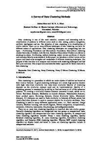
Distance Metrics and Clustering Methods for Mixed-Type Data Alexander H. Foss1, Marianthi Markatou1, Bonnie Ray2 1

Department of Biostatistics, 706 Kimball Tower, University at Buffalo, Buffalo, NY 14214, USA i 2 Arenadotio, New York, NY, USA Summary In spite of the abundance of clustering techniques and algorithms, clustering mixed interval (continuous) and categorical (nominal and/or ordinal) scale data remains a challenging problem. In order to identify the most effective approaches for clustering mixed-type data, we use both theoretical and empirical analyses to present a critical review of the strengths and weaknesses of the methods identified in the literature. Guidelines on approaches to use under different scenarios are provided, along with potential directions for future research. Keywords: Discretization, Dummy coding , Gower’s distance , k-means clustering, Machine learning, Mahalanobis distance, Mixture model, Multivariate data analysis, Unsupervised learning 1

Introduction

Cluster analysis, a type of unsupervised learning, is a widespread multivariate technique for exploratory data analysis and data summarization. It is characterized by a search for a latent categorical variable that explains a “meaningful” amount of the variability in a given data set. The levels of the latent variable are typically interpreted as denoting membership in distinct “clusters,” and the precise definition of “meaningful” varies widely with the particular type of cluster analysis being performed; for example, k-means clustering seeks to minimize the within-cluster variance (Hastie et al., 2009). With a few notable exceptions such as modal clustering (Li et al., 2007) and mixture models (Hunt and Jorgensen, 2011), cluster analysis often depends on distance functions to quantify (dis)similarity between points in the feature i

Author A. Foss is currently employed at Sandia National Laboratories; the manuscript was completed at, and funded by, the University at Buffalo

Distance Metrics and Clustering Methods for Mixed-Type Data

2

space; many clustering procedures are based on the goal of minimizing the distance between units in the same cluster while simultaneously maximizing distance between units in different clusters. What characteristics define an ideal cluster remains a challenging question, as in practice clusters can vary in shape, size, and density (Jain, 2010). A commonly invoked definition of an ideal cluster is a set of points that is compact and isolated, that is, a set of points that are similar to each other and well-separated from points not belonging to the cluster (e.g. see Cormack, 1971; Gordon, 1981; Jain, 2010; McNicholas, 2016a). Additional characteristics of clusters that may be desirable depending on the context are given in Hennig (2015b, Sect. 3.3), including stability of the identified clusters, independence of variables within a cluster, and the degree to which a cluster can be well-represented by its centroid. Both Hennig (2015b) and McNicholas (2016a,b) present thorough and incisive discussion related to the nature of cluster analysis, and the selection of appropriate clustering techniques. Both state that there is no single “best” clustering method in a general sense, but rather clustering techniques must be carefully selected in the context of the data at hand. Both discuss the fact that differing goals may also inform the choice of an appropriate technique; McNicholas (2016a,b) draws a distinction between clustering and dissection, i.e., the process of dividing homogeneous data sets into groups despite the absence of clear cluster structure, while Hennig (2015b) distinguishes between three possible goals of (1) exploration, (2) data reduction, and (3) comparison of clusters to other features of interest associated with a data set. McNicholas (2016a,b) argues that model-based clustering is generally preferable to alternative approaches for several reasons, including the usefulness of soft partitions and model averaging for handling multiple clustering results, the ability to perform appropriately when the number of modes is greater than the number of clusters, the existence of very broad parametric families that can be leveraged in the context of model selection, as well as clarity in communicating results to collaborators. Hennig (2015b), on 2


3

the other hand, is more agnostic with regard to choice of clustering technique, stating that the choice must be made pragmatically based on the context of the problem and data set at hand. Hennig (2015b) questions the very concept of a single “true” clustering, citing various mutually exclusive definitions and goals of clustering. Hennig instead offers a constructivist approach which emphasizes the pragmatic selection of a clustering technique based on the desired characteristics of a cluster, as well as the applied goals and data structure under consideration. Although Hennig avoids recommending any method be favored or avoided, problems with model-based methods are discussed, including sensitivity to deviations from the selected model, as well as the fact that some distributions are not technically feasible as component distributions due to identifiability requirements. In this paper we focus on clustering mixed-type data, that is, data sets with both interval (continuous) and categorical (nominal and/or ordinal) scale variables. Mixed data sets are ubiquitous across many disciplines, and with the advent of so-called “big data” the availability of data sets comprised of heterogeneous sources and data types will continue to increase (Fan et al., 2014). Many commonly used approaches involve strategies to adapt existing techniques for single-type data for use with mixed-type data. For example, if interval scale variables are discretized, clustering techniques for categorical data may be used (see Section 2.1), or if categorical variables are dummy coded, techniques for interval scale data may be used (see Section 2.2). We identify significant problems with these approaches below, and discuss techniques that have been explicitly designed to accommodate the unique challenges associated with mixed-type data, such as distance metrics for mixed-type data (Section 3) and statistical mixture models (Section 4). As we discuss in later sections, the fundamental challenge of equitably balancing the contribution of interval and categorical scale variables leads many existing approaches to fail. A method that does not equitably balance interval and categorical scale variables can fail even if one or the other variable type contains near perfect information. In some cases, statistical mixture models are able to 3


4

overcome this challenge of equitable treatment, although concerns regarding appropriateness of parametric assumptions are a significant difficulty in this area. Conclusions and further research directions are discussed in Section 6. While recognizing that there are a plethora of perspectives and definitions of clusters, we often invoke the mixture model perspective to shed light on various challenges of cluster analysis in the current paper. The mixture model perspective is particularly effective in this context as it (a) produces mathematically rigorous generative models for Monte Carlo studies (b) can naturally accommodate multiple data types (interval, discrete, etc.) without transformations or approximations (c) can handle dependencies within and between variable types, and (d) is flexible enough to capture a very wide range of scenarios of practical significance. The use of statistical mixture models to study latent classes (i.e. cluster structure) continues a long line of mathematics and statistics research, perhaps beginning with Pearson (1894). Further discussion and historical perspective can be found in McNicholas (2016a,b); various sources therein describe the primacy of the mixture model perspective in clustering, e.g., Marriott (1974) and Aitkin et al. (1981). Nevertheless, it is clear that clustering is not always about recovering mixture components. As pointed out in Hennig (2015b), the definition of a cluster is highly dependent upon the context of the problem and the available data. (Similarly, McNicholas (2016a) states that a cluster’s meaning depends upon the context of the data.) Clusters can be defined, for example, as zones of concentration of probability mass (Hartigan, 1975; Wishart, 1969), and in this sense, each cluster can be understood as a domain of attraction of a mode (Chacón, 2015; Stuetzle, 2003), or as partitions induced by level-sets of a density (Li et al., 2007; Rinaldo et al., 2012). These alternative perspectives may shed further light on the challenge of clustering mixed-type data; while we have used the parametric mixture model perspective to illustrate various points in the current manuscript, we in no way mean to imply that other perspectives should be rejected.

4


2

5

Data Transformation Approaches

In this section, we discuss strategies that involve transforming a mixed-type data set so that it can be clustered using existing methods designed for single-type data. Mixed-type data are data obtained as realizations of both interval and categorical scale random variables. First we discuss discretization of interval scale random variables and the use of clustering methods appropriate for categorical variables. Next, we discuss numerical coding in conjunction with interval scale clustering methods. 2.1

Discretization

Discretization of interval scale variables is a widely used strategy in many areas of statistics and machine learning, and the strengths and weaknesses of existing discretization methods have been previously discussed (Dougherty et al., 1995). In the discretization approach for clustering mixed-type data (e.g., He et al., 2005b), all interval scale variables are discretized, and a clustering method suitable for exclusively categorical data is applied (e.g. the k-modes algorithm (Huang, 1998) or latent class modeling (Goodman, 1974)). Although discretization is commonly used for clustering, it involves a potentially substantial loss of data resolution if the discretization uses inappropriate cut points (e.g., see Kerber, 1992, for a discussion in the context of classification algorithms). Clustering might be used to choose optimal cut-points (Dougherty et al., 1995), but this introduces potential circularity to the problem. Consider as an example a Monte Carlo study in which we cluster manifestations of the random vector (V, W ) defined by a mixture of two populations that are very well separated. Observations are drawn from the two populations in equal proportion according to    V ∼ N (0, 5.2),   V ∼ N (5.2, 5.2),

W ∼ M ultin(n = 1, p = (0.45, 0.45, 0.05, 0.05)), W ∼ M ultin(n = 1, p = (0.05, 0.05, 0.45, 0.45)),

5

if drawn from pop. 1 if drawn from pop. 2.


6

We generate samples of size N = 500 from this mixture distribution, discretize V as described below, and then cluster on W and discretized V using the k-modes algorithm (Huang, 1998) and latent class analysis algorithm (LCA, Hagenaars and McCutcheon, 2002) as implemented in the klaR (Weihs et al., 2005) and poLCA (Linzer and Lewis, 2011) packages in R. Additionally, a normal-multinomial mixture model as implemented in the flexmixedruns function of the fpc package (Hennig, 2015a) (which uses an underlying call to the flexmix package, Gr¨ un and Leisch, 2008) is used to cluster the original data prior to discretization. We drew 500 Monte Carlo samples for each number of bins for each clustering method. Discretization is either a median split into two bins, a tertile split into three, and so on up to nine bins. Figure 1 shows mean adjusted Rand index (ARI; Hubert and Arabie, 1985) for each of the discretization conditions. The k-modes algorithm performs best for a median split of the interval scale variable, and degrades as the number of cut-points increases, while the performance of LCA does not degrade as the number of cut-points increases. The normal-multinomial mixture model, which uses the untransformed interval scale variable, outperforms both competing algorithms for all choices of the cut-point. [Figure 1 about here.] In order to illustrate, in broad strokes, the relative performance of certain clustering methods, we report values of the adjusted Rand Index (ARI; Hubert and Arabie, 1985). We note that there exist many indices measuring clustering quality (Meila, 2005, 2007, 2016; Milligan and Cooper, 1986; Milligan, 1981; Strehl, 2000; Vinh et al., 2010), and that quality of clustering is multidimensional, depending upon the goals of clustering in the specific application. Our results were consistent on a variety of measures and ARI represents this agreement well. We note that in the current and subsequent experiments performance is generally meant as recovery of mixture components, although in some applications other measures of performance may be of interest. 6


7

The method of He et al. (2005a) involves clustering the interval scale variables separately from the categorical variables. The two resultant clusterings are combined into a single clustering result with the application of a clustering method suitable for categorical scale data. This approach is essentially a more extreme discretization method; instead of discretizing each interval scale variable separately, all interval variables are merged into a single discretized variable. 2.2

Numerical Coding Methods

Numerical coding involves converting categorical variables into numeric variables and clustering the newly formed dataset with methods suitable for interval scale data only, such as k-means (Hartigan and Wong, 1979). In some cases, there may be reasonable values that can be associated with each categorical level based on specific knowledge of the variable. For example, a variable representing the trichotomized income levels { 70000} could perhaps be replaced by the median income level within that categorical level. Often straightforward replacements are not possible, and other coding schemes must be used such as dummy coding and simplex coding (McCane and Albert, 2008). However, unlike regression, in which 0–1 dummy coding yields equivalent inferential results as 0–c dummy coding for any scalar c (after rescaling the estimated coefficient by 1/c), the specific choice of values can drastically impact the results of a cluster analysis. Thus, any such application of the numerical coding technique suffers from a non-trivial selection of c that determines the relative contribution of interval and categorical scale variables. There is no clear way to select c in an optimal manner. In practice, clustering with a numerical coding technique nearly always involves using 0–1 dummy coding with standardized continuous variables, with the idea that this represents an effective default choice in the absence of more information. Proposition 1 in Foss et al. (2016) illustrates the inadequacy of this default choice. Consider the general case of a bivariate

7


8

mixture distribution of two underlying populations, where the first variable is a mixture of two arbitrary continuous distributions with means 0 and µ and finite second moments, and the categorical variable is a Bernoulli mixture. Assume the squared Euclidean distance is calculated between an observation from population 1 and 2, with the standard practice of using 0–1 dummy coding and z-normalizing the interval scale variable. Proposition 1 in Foss et al. (2016) states that the expected contribution from the interval scale variable (defined as the expected value of the squared Euclidean distance within the interval scale variable) will always be greater than 1, while the expected contribution from the categorical variable will always be less than 1. Depending on the specifics of the data distributions used, often the contribution of the interval scale variable is many times that of the categorical. Thus, 0–1 coding is not generally an effective strategy for equitably balancing the contribution of interval and categorical scale variables to the overall clustering. In any specific case it may be possible, although not always easy, to select a weight c that balances contribution between interval and categorical variables. However, performance will be strongly dependent on known factors (e.g. the number of variables or the distance function used) and generally unknown factors (e.g. the amount of overlap between the clusters). We can conclude from these results that it is impossible to make an “optimal” choice of c that will apply with any generality across different data sets or clustering techniques; by this we mean that a choice of c that provides desirable performance in one scenario will fail in many other scenarios. It is important to note that standardizing all variables (i.e. dividing by their standard deviation or range) amounts to a similar choice of weights that may be acceptable in certain restricted settings, but is not ideal in any general sense. The following example illustrates the dependency of this approach on the choice of c in the context of k-means clustering, one of the most popular data mining algorithms (Wu

8


9

et al., 2008). Let (V, W ) denote a vector of random variables, where

V ∼

   N (0, 1)

if Z = 1 (1)

  N (µ, 1) if Z = 2, for µ ≥ 0, and where Z is a discrete random variable denoting population membership, taking on values 1 and 2 each with probability 0.5, and

W =

   cB

if Z = 1

  cB2

if Z = 2,

1

(2)

for c > 0, B1 ∼ Bern(0.5 − p), B2 ∼ Bern(0.5 + p), and p ∈ [0, 0.5]. Note that c represents a user-specified weight as used in dummy coding, and that local independence holds, that is, V 6⊥ W , but (V ⊥ W ) | Z, where “⊥” denotes independence. We now demonstrate that the k-means distance function captures information parametrized by p, but depends on the choice of c. If we denote the ith centroid selected by the k-means algorithm as (αi , βi ), then the squared Euclidean distance from an arbitrary point (v, w) to the centroid is given by

di = δE ((v, w), (αi , βi )) = (v − αi )2 + (w − βi )2 .

(3)

In order to further illustrate the behavior of k-means clustering, we plot in Figures 2, 3, and 4 values of d1 /(d1 + d2 ) for various values of µ, p, c, and (v, w) (for additional simulation details please see Appendix A.2). A ratio less than 0.5 indicates that the point (v, w) is closer to the centroid corresponding to cluster 1 versus the centroid of cluster 2. We see in these plots that the distances are strongly affected by µ, but that the relative influence of µ and p depends on the choice of c. When p = 0.5, w contains perfect information regarding cluster membership, but µ continues to have a greater influence on the distances even for 9


10

c = 2, the highest setting of c used. Lower settings of c are even less influenced by w. In this simulation and subsequent ones, we have constructed a true latent categorical variable corresponding to cluster membership. On pp. 55–56 Hennig (2015b) discusses the limitation of such a model, noting for example that data sets often can be partitioned in multiple distinct meaningful ways, and that multiple clustering approaches may also yield valid, but distinct, information. Our simulation setup is not designed to capture all such intricacies found in the real world, but rather to illustrate in an essentialized form our core findings. [Figure 2 about here.] [Figure 3 about here.] [Figure 4 about here.] We now proceed to give an additional example illustrating the fact that 0-c coding is suboptimal for any fixed choice of c, in the context of the k-means algorithm. We consider clustering a sample from a bivariate random vector (V, W ) that follows a mixture of two populations in equal proportions according to    V ∼ N (0, 1),

W ∼ M ultin(n = 1, p = (0.5 − , 0.5 − , , )),

if drawn from pop. 1

  V ∼ N (µ, 1),

W ∼ M ultin(n = 1, p = (, , 0.5 − , 0.5 − )),

if drawn from pop. 2

where µ ∈ R and ∈ [0, .25) were varied in order to systematically control the difficulty of the clustering problem. (The separation between population 1 and 2 decreases as µ → 0 or as → 0.25.) We quantified the separation between clusters using the concept of overlap in distributions (as used in e.g. Maitra and Melnykov, 2010), which consists of calculating the area of overlap 10


11

between the cluster densities (or mass functions for categorical variables). That is, the overlap between clusters with densities f1 and f2 in equal proportion is given by Z

Z f1 (t)dt +

A1

f2 (t)dt,

(4)

A2

where A1 = {x : f1 (x) < f2 (x)} and A2 = {x : f2 (x) < f1 (x)}. This generalizes in a straightforward manner to categorical random variables. Note that an overlap of 0% indicates complete separation, i.e. an easy clustering problem, while an overlap of 100% indicates an impossible problem since the clusters completely overlap. Although there are other ways to quantify cluster separation, such as average distance between centroids, or expected within- to between-cluster sums of squares, we found overlap to be the most direct, useful, and concise approach. We consider three clustering strategies: k-means with squared Euclidean distance and 0-1 dummy coding, k-means with squared Euclidean distance with 0–2 dummy coding, and a normal–multinomial mixture model as implemented in the fpc package in R 3.0.0. We use overlap levels of 1%, 15%, and 30% for both the interval and nominal scale variables, and measured performance using the ARI. We drew samples of size 500, with 1000 Monte Carlo samples drawn for each cell. Monte Carlo error was less than 0.01 in all cases. Results are shown in Table 1. As expected from the previous discussion, k-means with 0-1 dummy coding relies primarily on the interval scale variables, and is minimally affected by the nominal variables. This is demonstrated by the large changes in ARI across different levels of interval scale variable overlap, but relatively small changes in ARI across different levels of nominal-variable overlap. The arbitrarily chosen 0–2 coding improves this apparent lack of balance between interval and nominal scale variables that was observed for 0–1 coding, but at the cost of decreased performance in the high nominal-variable overlap conditions. 11


12

There exists some c, which we denote c∗ , such that 0–c∗ coding would offer the most balanced performance in this particular dataset, that is, performance in the (1% interval, 30% nominal) error condition equal to the (30%, 1%) error condition. However, even if c∗ were known, ML-EM (Maximum-Likelihood estimation using the EM algorithm) of the finite mixture model would still outperform the k-means technique. If we examine the (30% interval, 1% nominal) overlap conditions, we see that k-means 0–2 coding still performs worse than ML-EM of the the mixture model; thus, c∗ is greater than 2. However, even with c = 2, ML-EM of the mixture model still outperforms k-means with 0–2 coding in the (1% interval, 30% nominal) condition, a margin of difference that would only increase for c > 2. We conclude that even if c∗ could be identified, it would still result in undesirable algorithm performance relative to the finite mixture model. This example, along with the results of the previous discussion, illustrates the fundamental flaw with any approach that requires user-specified weights, including the numerical coding and hybrid distance techniques described below. We acknowledge that manually weighted methods continue to be a useful technique when weights can be selected in a rigorous and justifiable manner based on a priori knowledge; however, in the absence of clear guidance, commonly used default weights can lead to unintended consequences. Several approaches have used dimension reduction techniques for mixed-type data in the numerical coding context. Dimension reduction techniques for nominal or mixed-type data (e.g., de Leeuw and Mair, 2009; Pages, 2004) can potentially be used to collapse variables of distinct types into newly constructed interval scale variables designed to explain the maximum possible variance in the original data. Morlini (2012) used tetrachoric correlations to estimate a full correlation matrix between interval and binary scale variables, and then used PCA to construct interval scale variables; a similar approach has been suggested using multidimensional scaling (Azzalini and Menardi, 2014). Caution is required when applying dimension reduction in cluster analysis: as Chang (1983) noted, applying dimension reduc12


13

tion to a data set can discard useful information regarding the latent cluster structure. The method of Honda et al. (2007) seeks to avoid this potential difficulty by applying PCA locally within each cluster. Although these methods may yield sensible weightings within categorical variables, they do not address the underlying problem of identifying equitable weights between interval and categorical scale variables. Although it is designed for interval scale data only, the method of Bouveyron and Brunet (2012) perhaps suggests an interesting solution, in which a discriminant analysis is incorporated within the mixture model framework to simultaneously cluster and reduce the dimension of the data. [Table 1 about here.] 3

Hybrid Distance Methods

Hybrid distance methods involve selecting a distance function that can accommodate both interval and categorical scale variables. Then, the data is clustered using one of the myriad clustering methods that only depend on the data through the distance function (e.g., many of those discussed in Kaufman and Rousseeuw, 1990). A distance function defined on two probability distributions that has been used to construct distances for mixed-type data is the Kullback-Leibler divergence (Kullback and Leibler, 1951). For two probability measures F1 and F2 , with F1 absolutely continuous with respect to F2 , the Kullback-Leibler divergence is

Z dKL (F1 , F2 ) =

log

dF1 dF2

dF1 ,

provided that the Radon-Nikodym derivative of F1 with regard to F2 ,

(5)

dF1 , dF2

exists. The

quadratic distance (Lindsay et al., 2008; Markatou et al., 2016) is an extension of the chi-

13


14

squared measures of distance between two distributions, and has the form Z Z K(s, t) d(F1 − F2 )(s) d(F1 − F2 )(t)

dK (F1 , F2 ) =

where K(s, t) is some non-negative definite kernel (i.e.

RR

K(s, t)dσ(s)dσ(t) ≥ 0 for all

bounded signed measures σ). Although various distance metrics described below are based on the Kullback-Leibler distance, an open area for further research involves investigating the properties of metrics constructed from alternative distances, such as the quadratic distance. Prior statistical work has addressed the challenge of defining distance metrics between mixed-type distributions. The location model (Krzanowski, 1993; Olkin and Tate, 1961) considers the categorical variables to follow a multinomial distribution, and the interval scale variables to be multivariate normal conditional on the categorical state. The work of BarHen and Daudin (1995) derives a distance for the location model using the Kullback-Leibler divergence (Kullback and Leibler, 1951). Bedrick et al. (2000) proposed a similar distance for mixed interval and ordinal scale data, with ordinal variables modeled as discretized latent normal variables, while de Leon and Carriere (2005) extended the location model to accommodate mixed interval, ordinal, and nominal scale data. Using the general mixed-data model of de Leon and Carriere (2005), the distance between two distinct populations P (g) 0

and P (g ) of mixed nominal, ordinal, and interval scale is

d(P

(g)

,P

(g 0 )

S

S X

πgs X πgs + πg0 s + (µgs − µg0 s )> Σ−1 (µgs − µg0 s ) )= (πgs − πg0 s ) log 0s π 2 g s=1 s=1 +

S−1 X πgs + πg0 s s=1

2

(τ gs − τ g0 s )> R−1 (τ gs − τ g0 s ),

where categorical state s ∈ {1, ..., S} indexes the sth categorical state, and each categorical state is defined as a unique combination of the nominal variables, πgs denotes the probability

14


15

that state s is observed in population g, µgs denotes the mean of the observed interval scale variables at state s in population g with shared covariance matrix Σ, τ gs denotes the conditional mean of the latent normal variables conditioned on both the sth categorical state and µgs , and R denotes the matrix of conditional polychoric correlations of the ordinal variables. Note that mixtures of these location models and generalizations thereof are not identifiable without further conditions on the parameters (Willse and Boik, 1999); this issue is discussed in depth in Section 4. Krzanowski (1983) proposes an alternative distance based on Matusita’s distance (Matusita, 1967). The work of Liu and Rubin (1998) proposes extending the location model with structured covariance matrices or by replacing Gaussian distributions with t-distributions. The location model and its generalizations have been used for hypothesis testing (de Leon, 2007; Krzanowski, 1984), discriminant analysis (de Leon et al., 2011; Krzanowski, 1980, 1982), and for mixture modeling of mixed-type data (Lawrence and Krzanowski, 1996). Finite mixtures of location models are discussed below in Section 4. A popular hybrid distance function is Gower’s distance (Gower, 1971). The distance between two vectors x and y of length m is calculated as follows. Let fj (xj , yj ) := |xj − yj |/rj if xj and yj are interval scale (where rj gives the sample range of variable j) and let fj (xj , yj ) := I{xj 6= yj } if xj and yj are categorical (where I is the indicator function). Then Gower’s distance is Pm dG (x, y) =

wj fj (xj , yj ) Pm , j=1 wj

j=1

where wj is a user specified weight for variables j = 1, 2, ..., m. In the absence of specific information, the weights in Gower’s distance are often set to 1. Just as with numerical coding strategies described above, it is difficult to choose the weights effectively, and a setting that works well in one scenario is not guaranteed to work well in others. Additionally, the categorical distance function used in Gower’s distance is insensitive to the probabilities of each categorical level within clusters, which further limits its effectiveness in handling

15


16

mixed-type data. The following example illustrates these flaws in Gower’s distance when used in conjunction with PAM (a k-medoids algorithm, Kaufman and Rousseeuw, 1990). Specifically, we show that the distance function remains unchanged as the underlying categorical level probabilities change for each cluster, a problem that does not apply to k-means with dummy coding or normal-multinomial mixture models. Consider the model described in Equations 1 and 2. If we denote the ith medoid selected by PAM as (αi , βi ), then Gower’s distance from an arbitrary point (v, w) to the ith medoid is

gi = δG ((v, w), (αi , βi )) = γ1

|v − αi | + γ2 I{w 6= βi }, r

(6)

where γ1 and γ2 are user-specified weights, r is the sample range over the observations of the interval scale variable, and I{·} is the indicator function. Figure 5 illustrates the behavior of PAM/Gower clustering, and depicts values of g1 /(g1 +g2 ) for various values of µ, p, and (v, w) (for additional simulation details please see Appendix A.2). We assume that the weights γ1 and γ2 are set to 1. We see in these plots that the distances are almost completely insensitive to p, and that the overall distance is dominated by the value of w. When p is low, the value of w gives no information whatsoever regarding cluster membership, and yet PAM/Gower still is strongly affected by w in this case. [Figure 5 about here.] The k-prototypes algorithm (Huang, 1998) is another popular clustering strategy that uses the hybrid distance technique. It uses a distance function very similar to Gower’s distance, except that squared Euclidean distance is used for the interval scale variables. The clustering stage proceeds analogously to that of k-means. The distance between observations

16


17

(v1T , w1T )T and (v2T , w2T )T used in k-prototypes is

dcon (v1 , v2 ) + γdcat (w1 , w2 ),

(7)

where vi and wi are vectors of interval and categorical scale variables, respectively, for the ith data point, and dcon and dcat are the continuous and categorical distance functions (in this case set to squared Euclidean and matching distance). Unlike Gower’s distance, k-prototypes does not allow variable-specific weights; rather, a single weight γ is used to weight the entire categorical contribution to the distance function. This weight, like those involved in dummy coding and Gower’s distance, is again either difficult or impossible to choose optimally. Other hybrid distance metrics have been proposed in the literature (e.g., Ahmad and Dey, 2011; Cheung and Jia, 2013; Hennig and Liao, 2013), in which similar challenges arise in choosing appropriate weights to control the relative contribution of interval and categorical scale variables. Section 2.1 of Foss et al. (2016) discusses the method of Hennig and Liao (2013) in more detail. Modha and Spangler (Modha and Spangler, 2003) develop a method very similar to the k-prototypes framework. Notably, they develop a method for estimating a suitable weight γ that scales the relative contribution of the interval and categorical scale variables. Their method proceeds as follows (note that we make use of the terminology defined in equation 7). First, they define the average within-cluster distortion separately for interval and categorical scale variables as Γcon =

G X

X

dcon (vi , cg,con )

g=1 {i:vi ∈ cluster g}

Γcat =

G X

X

dcat (wi , cg,cat ),

g=1 {i:wi ∈ cluster g}

where i = 1, 2, ..., N , and where cg,con and cg,cat denote centroids of the gth cluster for interval

17


18

and categorical scale variables. Centroid cg,con is defined as the sample mean within cluster P ¯ = v∈Cg v/ng , where Cg denotes the set of ng elements contained in cluster g, i.e. cg,con = v g. For a set of 0-1 dummy coded categorical variables wi in cluster Cg , cg,cat is defined as P S(w)/||S(w)||, where S(w) = w∈Cg w and || · || denotes the L2 norm. They define the average between-cluster distortion as

Λcon =

N X

dcon (vi , c¯con ) − Γcon

i=1

Λcat =

N X

dcat (wi , c¯cat ) − Γcat ,

i=1

where c¯con and c¯cat are the centroids taken across all interval or categorical scale variables, respectively. Finally, they define the objective function as

Q=

Γcon Γcat · . Λcon Λcat

The Modha-Spangler algorithm then uses a brute-force search to cluster repeatedly for a range of values of γ, and selects the γ that minimizes Q. In many situations, Modha-Spangler clustering is able to equitably balance the contribution of interval and categorical scale variables, unlike any other hybrid distance technique; often this leads to excellent performance. However, the method performs poorly in certain situations. For example, if the number of clusters is chosen to equal the number of non-empty cells in the cross-tabulation of the categorical variables, the method will simply allocate the observations in each cell to a unique cluster, regardless of the interval scale variables. This occurs because the allocation yields a Γcat of zero, which leads to a Q equal to zero, which appears to be a “perfect” minimization of Q. This is illustrated in simulation B of Foss et al. (2016). Simulation A of Foss et al. (2016) illustrates additional conditions in which the

18


19

method of Modha-Spangler underperforms relative to competing methods due to an overreliance on interval scale variables. A further limitation of the k-prototypes method and the Modha-Spangler method arises from the fact that the single weight γ does not allow individual variables to be up- or downweighted, leaving both algorithms vulnerable to individual noninformative variables. See Table 2 and associated discussion in Section 4 for an example of this problem in Modha-Spangler clustering. Statistical distances, because they are based on distributions, are used with a variety of models, including that of de Leon and Carriere (2005). Although statistical distances are constructed based on an explicit data generation model, non-statistical distances are generally not (including, e.g., the aforementioned Gower’s distance, the distance used by k-prototypes, and the Modha-Spangler technique). 4

Statistical Mixture Models

Statistical methods involve the use of a parametric model for the joint distribution, typically in the form of a finite mixture model (Everitt and Hand, 1981; McLachlan and Basford, 1988; McLachlan and Peel, 2000; McNicholas, 2016a; Titterington et al., 1985). For example, in a Gaussian mixture model (Banfield and Raftery, 1993; Fraley and Raftery, 2002; Scott and Symons, 1971; Wolfe, 1965, 1970), the data vectors Xi to be clustered are assumed to be drawn from one of G possible Gaussian distributions, that is, Xi ∼ N (µj , Σj ), j = 1, 2, ..., G P with probability πj , where G g=1 πg = 1 and 0 < πg ≤ 1 ∀ g. The associated density of Xi P is fXi (t) = G g=1 πg f (t; µg , Σg ), where f is the normal density. There is a rich variety of distributions that have successfully been used as component distributions in finite mixture modeling of interval scale variables, including the beta (Ji et al., 2005), gamma (Mayrose et al., 2005), skew normal (Lin, 2009; Lin et al., 2016), skew t (Lee and McLachlan, 2014; Lin and McLachlan, 2010; Murray et al., 2014; Vrbik and McNicholas, 2014), generalized hyperbolic distributions (Browne and McNicholas, 2015), normal-inverse Gaussian (Karlis

19


20

and Santourian, 2009), shifted asymmetric Laplace (Franczak et al., 2014), as well as copulas for modeling more general families of non-independent interval scale variables (Ghosh et al., 2011; Kosmidis and Karlis, 2016). Mixture models have been successfully applied to nominal, ordinal, and count data as well (Cai et al., 2011; Fernandez and Arnold, 2016; Fong and Yip, 1993; Foss et al., 2016; Hunt and Jorgensen, 2011; Vermunt and Magidson, 2002). The parameters of finite mixture models are generally estimated using some variant of the EM algorithm (Dempster et al., 1977). Well-known limitations of the EM algorithm include vulnerability to getting “trapped” in local maxima of the objective function (thus requiring multiple initializations), possibly intractable integrals in the E step (possibly requiring multidimensional numerical integration), and possibly undefined objective functions on the boundary of parameter space (e.g., variance σ ˆ 2 = 0 of a mixture model component). In the discussion below, we show that finite mixture models are often able to overcome the challenge of balancing interval and categorical scale contribution, but can deliver poor performance when parametric assumptions are strongly violated. Non-parametric density-based methods (Azzalini and Torelli, 2007; Chacón, 2015; Esther et al., 1996; Li et al., 2007; Rinaldo et al., 2012; Wishart, 1969), and the closely related meanshift algorithm (Comaniciu and Meer, 2002), have been proposed that relax the assumptions inherent to parametric model-based clustering methods. However, the multivariate density estimation step incurs a prohibitively large computational cost with even a modest number of interval scale variables, in addition to problems of overfitting the data (Scott, 1992, Chapter 7). Additionally, these kernel density methods require interval-scale data and are not generally suited for mixed-type data. The TwoStep algorithm (Chiu et al., 2001) is an agglomerative hierarchical algorithm that assumes a mixture distribution of joint normal-multinomial components. It involves an initial pre-clustering step similar to the BIRCH algorithm (Zhang et al., 1997), and uses a distance function based on the decrease in the overall log-likelihood upon merging two 20


21

clusters. Since it only requires a single pass through the data, the TwoStep algorithm is extremely computationally efficient. However, the efficient performance naturally comes at the cost of the quality of the solution obtained. Unless the data set to be analyzed is truly too large to be processed more than once, this method is not recommended. Since iterative methods such as EM estimation schemes for finite mixture models can often yield very good solutions in a manageable number of iterations, these methods should not be disregarded for very large datasets. A common mixture model used for mixed-type data is the normal-multinomial mixture model (Fraley and Raftery, 2002; Hunt and Jorgensen, 2011), with the distribution of Xi = (Vi T , Wi T )T given cluster membership set to the joint normal-multinomial distribution, i.e.

fXi (x) =

G X

πg fg (x; µg , Σg , pg1 , pg2 , ..., pgQ ),

g=1

with

fg (vi , wi ; µg , Σg , pg1 , pg2 , ..., pgQ ) = φ(vi ; µg , Σg )

Q Y

M ultin(wiq ; n = 1, pgq ),

q=1

where Vi is multivariate normal given group membership, Wi is a vector of Q nominal variables which are conditionally multinomial given group membership, where Wiq takes on the values {1, 2, ..., Lq }, φ is the multivariate normal density, and M ultin(·) is the multinomial mass function, where M ultin(wiq ; n = 1, pgq ) = pgqj , with j = wiq . A key consideration in specifying a mixture model is whether the variables are conditionally independent within a cluster, a property referred to as local independence (e.g., Hennig and Liao, 2013). Previous work relating to categorical and nonparametric continuous latent class models has shown conditional independence to be an important property often required for identifiability (Allman et al., 2009). Various formulations of the joint normal-multinomial

21


22

model have been proposed depending on the within-cluster dependence structure that is employed. The model above assumes within-cluster dependence within the interval but not within the nominal scale variables, and conditional independence between interval and nominal scale variables. Dependencies within the nominal variables can be specified by defining a Q new nominal variable with Q q=1 Lq levels, where each level in the new variable corresponds to a unique combination of the original nominal variables’ levels. Specifying conditional dependence between interval and nominal scale variables can be accomplished using the method of Everitt (1988), in which the nominal variables are discretized interval scale variables with a flexible covariance structure. For nominal variables with more than two levels, this imposes ordinal structure of the levels, and requires numerical integration that is computationally impractical for a large number of nominal variables (Everitt and Merette, 1990; Willse and Boik, 1999) since the time complexity of m-dimensional cubature grows exponentially in m (Cools, 2002). A similar approach proposed by McParland and Gormley (2016) can accommodate mixed interval, ordinal, and nominal scale variables, in which ordinal variables are assumed to arise from discretized normal mixtures, and the nominal variables arise from discretized multivariate normal mixtures. This approach offers a flexible set of specifications for the covariance structure of the latent normal mixtures, although currently the authors restrict their attention to diagonal covariance structure for the latent variables; this restriction could be lifted, but it would introduce the aforementioned challenge with exponential time complexity. Browne and McNicholas (2012) propose a related latent variable model which uses a factor model to relate the observed interval scale variables to the latent variables, and a latent trait model to relate observed nominal variables to the latent variables. A distinct factor/latent trait model is assumed between the latent variables and the observed variables for each cluster, with observed variables assumed to be conditionally independent given the latent variables and given cluster membership (this explicitly allows for dependence given cluster but unconditional on latent variables). The model is fitted using the EM algorithm, 22


23

and like other latent variable models described above, involves computationally expensive numerical techniques to approximate intractable integrals. An alternative approach for handling within-cluster dependencies between interval and nominal scale variables proposed by Lawrence and Krzanowski (1996) uses a mixture of location models (e.g., Krzanowski, 1993; Olkin and Tate, 1961) in which the interval scale variables are modeled as multivariate normal with unique parameters for each cluster and categorical state. For a vector of random variables (V , W ), where V is a vector of continuous random variables and W is a Q × 1 vector of nominal random variables with Lq categorical levels in variable q ∈ {1, 2, ..., Q}, the location model first defines a categorQ ical random variable Z ∈ {1, 2, ..., S = Q q=1 Lq } where each of the S categorical states corresponds to a unique combination of the original nominal variable levels in W . Then (V , W ) is modeled as V | Z = s ∼ N (µs , Σs ) within state s as determined by W , with associated density f (v, w | θ) = h(v | Z = s, θ)P r(Z = s), where h is the multivariate normal density with mean µs and covariance matrix Σs as indexed by the state of Z, and θ = (µ1 , µ2 , ..., µS , Σ1 , Σ2 , ..., ΣS ). A mixture of location models states that each vector (V , W ) arises from one of G location models, with group membership g ∈ {1, 2, ..., G} P unknown, with the overall mixture density function given by f (v, w) = G g=1 πg fg (v, w | θ g ). One obvious limitation of the location model is that the number of combinations of categorical levels increases exponentially in the number of nominal variables. For most data sets with multiple nominal variables, this inevitably leads to small sample sizes within each categorical cell. Consider two typical mixed-type data sets analyzed in Foss and Markatou (2018): the first, a biomedical data set, contains five nominal variables measured on 475 patients, while the second contains five nominal variables measured on about 80 million domestic airline flights in the United States. The distribution of counts within the combinatorial cells for each data set is shown in Figure 6; in the biomedical data set the median number of observations per cell is two, and even in the much larger airline data set 25% of 23


24

the cells have count less than sixteen. Aside from computational issues that may arise due to the number of estimated parameters increasing exponentially in the number of nominal variables, a mixture of location models is not necessarily identifiable. Willse and Boik (1999) showed that a mixture of location models with equal covariance across cluster and categorical state is not identifiable without further restrictions on the conditional means, and propose models which allow a mean shift for each categorical state that is equal across clusters. This lack of identifiability applies to the location model and extensions, such as the general mixed-data model of de Leon and Carriere (2005). Special cases of identifiable location mixture models include the model that is defined by µgs = µg , ∀g, s, where g indexes the G groups, and s indexes the S categorical states as defined above, and the additive model. The additive model defines the conditional means as µgs = µg +θ s , where θ s denotes the difference in conditional means between location 1 with θ 1 = 0 and location s. This difference is assumed to be the same for all groups and introduces a parallel structure in the conditional means. These restricted location mixture models are identifiable, and the parallel structure simplifies the interpretation of fitted models in an applied setting. The first restricted model is essentially a local independence model in the sense that interval and nominal scale variables are independent conditional on group membership, and can be fitted by constructing Z as defined above and using standard software for local independence mixture models. Even the additional flexibility provided by the additive model, however, is quite far from the flexibility potentially offered by the full location model, and the parallel conditional mean structure may or may not be plausible based on the particular data set being analyzed. [Figure 6 about here.] While a full proof is given in Willse and Boik (1999), we provide here an illustration that shows some intuition behind the non-identifiability of unrestricted mixtures of location 24


25

models, along with practical limitations of using such a mixture. We begin with the standard definition of identifiability. Definition 1: A class D of mixtures is identifiable if and only if for all densities f ∈ D the equality of two representations of f G X

πg kg (x; θ g ) =

g=1

e G X

π ej kj (x; θej )

(8)

j=1

ej (Everitt and Hand, 1981, e and ∀ g ∃ j such that πg = π implies that G = G ej and θ g = θ Chapter 1, p. 5). For our current purposes, let the class D of mixtures denote the set of functions ) G X f f (v, w) = πg h(v|w)mg (w) g=1

( D=

where W |g ∼ M ultinomial(n = 1, pg ), pg is a q × 1 vector, W ∈ {1, 2, ..., Q}, mg (w) = pgw is the multinomial mass function for n = 1, and V |W = w, g ∼ N (µgw , Σgw ), with density h(v; µgw , Σ) (we assume for simplicity that Σgw = Σg0 w0 = Σ). In order to show that the class D of mixtures is not identifiable, it suffices to construct ej , g, j ∈ {1, 2, ..., G} in which Equation 8 holds but two sets of parameter vectors θ g and θ e does not hold as required by Definition 1. the correspondence between θ’s and θ’s Example: Here we provide an example of a two-component mixture of unrestricted location models that is unidentifiable. Consider exam scores taken from two classrooms of students, one an honors class and one standard. Suppose that exam scores are conditionally normal with unit variance given class and sex with means of the form µg,w , e.g., µboy,0 = 0, µgirl,0 = 1, µboy,1 = 2, and µgirl,1 = 4 where standard classroom is indexed by w = 0 and honors indexed by w = 1. If classroom is observed and sex is unobserved, then we might seek to separate

25


26

students by sex using the mixture model

f (v, w) = πgirl k(v, w; θ 1 ) + (1 − πgirl )k(v, w; θ 2 ) X (1−w) = πg φ(v − µg,w )pw g (1 − pg ) g∈{boy,girl}

where θ 1 = (µgirl,0 , µgirl,1 , pgirl ), θ 2 = (µboy,0 , µboy,1 , pboy ), φ denotes the standard normal density function, v denotes exam score, and pboy and pgirl denote the probability that a boy or girl, respectively, is enrolled in the honors class. e1 = (µboy,0 , µgirl,1 , p = Assume for simplicity that pgirl = pboy = p = 1/2 and πgirl = 1/2. Let θ e2 = (µgirl,0 , µboy,1 , p = 1/2). Then the mixture density f (v, w) = 1/2) θ 1 k(v, w; θ 2 ) 2

1 k(v, w; θ 1 ) 2

+

can be rewritten as     1 [φ(v − µ

girl,0 ) + φ(v − µboy,0 )] , 1 4 [φ(v − µgirl,w ) + φ(v − µboy,w )] =  4  1 [φ(v − µ  girl,1 ) + φ(v − µboy,1 )] , 4     1 [φ(v − µboy,0 ) + φ(v − µgirl,0 )] , 4 =    1 [φ(v − µgirl,1 ) + φ(v − µboy,1 )] , 4

if w = 0 if w = 1 if w = 0 if w = 1

e1 ) + 1 k(v, w; θ e2 ). Thus, by the definition of identifiability, which is equivalent to 21 k(v, w; θ 2 the mixture in this example is not identifiable. Practically speaking, a mixture in which each component corresponds to one sex is indistinguishable from a mixture in which the first component captures boys in the standard classroom and girls in the honors classroom, and the second component captures girls in the standard classroom and boys in the honors classroom. When parametric assumptions hold (a challenge we discuss further below), the locallyindependent normal-multinomial mixture model is often able to equitably balance the con-

26


27

tribution of interval and nominal scale variables. This property is illustrated in the following example, in which we investigate the specific form of the posterior probabilities emerging from a normal-multinomial mixture model. Compared to similar analyses above of the distance functions used in k-means and PAM/Gower, we show that only the mixture model is able to achieve a sensible balance between interval and nominal scale variables, while these alternative methods suffer from serious deficits in balancing the two data types. In the context of the model described in Equations 1 and 2, we show that ML-EM (Maximum-Likelihood estimation using the EM algorithm) of a normal-multinomial mixture model provides a similarity function that captures information parametrized by p and does not depend on the choice of c. We use the normal-multinomial mixture model, which in this case is

f (v, w; Ψ) =

G X

πg fg (v, w; θg ),

g=1

where θg = (µg , σg , pg ),

PG

g=1

πg = 1, πg > 0 ∀g, Ψ = (π1 , π2 , ..., πG , θ1 , θ2 , ..., θG ), and

fg (v, w; θg ) = φ

v − µg σg

pgI{w=c} (1 − pg )I{w=0} ,

where φ(·) is the standard normal density function and I{·} is the indicator function. Note in particular that these functions capture information parametrized by µ and p, but remain unchanged for different choices of c. For the ith observation, we estimate the probability of membership in the g th group as ˆ zˆg = Pˆ (ith observation ∈ population g | (v, w)i , Ψ) π ˆg fg ((v, w)i ; θˆg )

= PG

k=1

π ˆk fk ((v, w)i ; θˆk )

(9) .

Note that posterior probability membership can be interpreted as a similarity function be-

27


28

tween a point and a mixture component. Figure 7 depicts values of zˆ2 as given in eq. 9 for various values of µ, p, and (v, w) (for additional simulation details please see Appendix A.2). Note that a value of zˆ2 less than 0.5 indicates that the point (v, w) is closer to cluster 1 compared to cluster 2 (according to the estimated posterior probability). We see in these plots that ML-EM of the mixture model achieves a superior balance of the interval and categorical scale components based on how informative the variable is. When p = 0.5, the categorical variable contains perfect information with regard to cluster membership, and zˆ2 behaves appropriately: in this case zˆ2 is completely determined based on whether w = 0 (left plot) or w = 1 (right plot). On the other hand, when p is low, the categorical variable is mostly uninformative with regard to cluster membership, and zˆ2 behaves appropriately: in this case zˆ2 is primarily determined by the value of v and µ, and mostly unaffected by w. In particular, compare this behavior to that of the less effective k-means with dummy coding (Figures 2, 3, and 4) and PAM/Gower (Figure 5). Of these three methods, ML-EM of the mixture model is the only approach that performs reasonably well across the entire range of p, that is, it can flexibly adapt depending on how “useful” the categorical variable is relative to the interval scale variable. [Figure 7 about here.] Favorable properties of mixture models are further illustrated in a simulation, whose results are shown in Table 2. This simulation involves a collection of two interval and five binary variables, with two underlying clusters. One binary variable has 1% overlap, while the other binary variables have 99% overlap. The interval scale variables all have the same overlap, which is varied systematically from 1% to 45%. Sample size was N = 500, with 500 Monte Carlo samples drawn per cell. With this data structure, a method (such as k-means) that relies mainly on the interval scale variables will perform more poorly as the interval-scale variable overlap increases. A method such as Modha-Spangler clustering 28


29

that cannot identify and upweight the single binary variable with 1% overlap will also not perform well, as it is forced into “choosing” between relying on the interval scale variables, or on the collection of mostly uninformative binary variables. The finite mixture model is the only method able to effectively combine interval and categorical scale information and thus detect the association between the single binary variable with 1% overlap and the interval scale variables. Furthermore, only a method (such as the finite mixture model) that is subsequently able to selectively minimize the deleterious influence of the four binary variables with 99% overlap will be able to perform well. [Table 2 about here.] Despite the ideal performance we see from the finite mixture model in many situations, the important caveat here is that the parametric assumptions must be reasonable. As an example, consider a simulation study whose results are shown in Table 3. This simulation consisted of datasets with 6 through 54 variables depending on the simulation condition, half interval and half nominal scale. Two interval and two nominal scale variables in every condition had 1% overlap, while the remaining variables had 99% overlap. The interval scale variables with 99% overlap followed a (highly skewed) normal-gamma convolution distribution; see Appendix A.3 for more details. Sample size was N = 500, with 500 Monte Carlo samples drawn per cell. We see here a breakdown of ML-EM (Maximum-Likelihood estimation using the EM algorithm) of the normal-multinomial finite mixture model with diagonal covariance matrix, as the distributional assumptions made by the model are severely violated by skewed data. ML-EM of a normal-multinomial mixture model with equal spherical covariance structure performs better, but is outperformed by k-means using Hennig-Liao weighting (Hennig, 2015b) and Modha-Spangler clustering (Modha and Spangler, 2003). These latter two methods perform comparably for a smaller number of uninformative variables, but Modha-Spangler performs better for a larger number of uninformative variables. 29


30

The Modha-Spangler algorithm is the top performer here, as it is able to successfully identify the weight that equitably combines the interval and nominal scale variables, even as they are obscured by increasing numbers of uninformative variables. Although it is often true that a distribution can be approximated well if the number of components is sufficiently large, an excessive number of clusters does not generally provide parsimonious or useful information about meaningful subgroups in the data. Thus, it is always desirable to select distributions that fit the underlying clusters well; if the true distribution deviates excessively from the assumed distribution, the performance of any parametric method will generally suffer. [Table 3 about here.] As mentioned above, kernel density based methods can be used to relax the parametric assumptions. However, in addition to the problems discussed above, categorical variables do not satisfy the continuity requirements inherent to the approach. One potential strategy has been proposed for incorporating categorical variables into a kernel-density clustering framework by (Azzalini and Menardi, 2014). This approach involves using a hybrid distance function to construct a dissimilarity matrix using the full dataset, which is then used to map the units onto a D-dimensional Euclidean space using multidimensional scaling, for some manageable dimension D. The D-dimensional data is then clustered using the density-based method. This approach is in fact an example of the hybrid distance method discussed in Section 3, with all of the associated limitations. Foss et al. (2016) develop an alternative method KAMILA (KAy-means for MIxed LArge data) for relaxing the parametric assumptions of mixture modeling using kernel density estimation. For a vector of continuous random variables X spherically symmetric around a center µ, proposition 2 in Foss et al. (2016) states that the probability density function of X can be expressed as fR (r) Γ( p2 + 1) , fX (x) = prp−1 π p/2 30

(10)


where R =

31

p (X − µ)> (X − µ), and fR is the probability density function of R. Under the

assumption that individual clusters are spherical, Eq. 10 can be used to model individual clusters, and univariate kernel density estimation is used to construct an estimate of the density of R as fˆR . By substituting fR with fˆR , we thus obtain the cluster density function fˆX . Note that this process can be extended to elliptical clusters through the use of a scaling matrix Σg that can be specified to be distinct or equal for each cluster. Currently nominal variables are modeled as multinomial within each cluster, although KAMILA is agnostic regarding this specification and can accommodate any choice of probability distribution. The cluster-specific parameters of the interval and nominal scale variables are estimated through an iterative procedure similar to the EM algorithm, and at the tth iteration the kernel density estimate of fR is constructed as N 1 X (t) ˆ k fR (r) = N h(t) i=1

(t)

r − ri h(t)

! ,

where N is the sample size, k(·) is the kernel function with corresponding bandwidth pa(t)

rameter h(t) at iteration t, and ri is the Euclidean distance between the ith observation and the nearest centroid µ(t−1) from the previous iteration. Details of the estimation procedure are given in Foss et al. (2016). As described in Foss et al. (2016), KAMILA does not require discretization of interval scale variables or dummy coding of nominal variables, and tends to achieve a favorable balance between interval and nominal scale variables comparable to traditional finite mixture models. Furthermore, KAMILA outperforms normal-multinomial mixture models in both skewed and heavy-tailed interval scale cluster distributions. The added flexibility of KAMILA comes at the cost of performance for small sample sizes (e.g., smaller than 100, although this depends heavily upon the number and overlap of the clusters, and the number of variables). If the true distribution of the clusters is known then it is generally preferable to use the correct distribution rather than a semiparametric approxi31


32

mation. As with other mixture models relying on a multinomial model, an excessive number of categorical levels in the nominal variables requires a commensurate sample size (although the specific number depends upon the overlap in the distributions). If an inadeqate sample size is suspected, KAMILA incorporates a categorical smoother that can ameliorate these issues in most circumstances. The KAMILA method has been implemented in the R package kamila, as well as in Hadoop, with usage recommendations described in Foss and Markatou (2018). 5

Model Selection and the Number of Clusters

Despite the popularity of clustering methods, selecting the number of clusters G remains a difficult problem. This is essentially an instance of the more general model-selection p problem. A rule specifying G = n/2 was proposed by Mardia et al. (1979). While such a straightforward rule may be more or less desirable depending on the problem at hand, this method is easily applicable to both single- and mixed-type data sets. Another approach is to select the smallest G that yields a “relatively” large criterion (e.g., SAS, documentation usage note 22540) for some internal measure of cluster validity. What constitutes the best choice of internal measure and threshold is generally unclear; furthermore, how one defines “best” in the first place is dependent upon the particulars of the data set and clustering goals (Hennig, 2015b). Some guidance may be provided by the empirical studies of Milligan (1981) and Milligan and Cooper (1985). Due to the fact that many internal measures require the selection of a distance metric, this approach introduces all of the complications of selecting weights, coding strategies, or hybrid distance metrics as discussed in Sections 2.2 and 3. For model-based methods with a valid likelihood function, selection of G and/or variable selection may be performed by maximizing a penalized likelihood measure such as AIC (Akaike, 1974), BIC (Schwarz, 1978), AICMIX (Hui et al., 2015), ICL (Biernacki et al., 2000), MICL (Marbac and Sedki, 2017), or QIC (Dimova, 2010). This method is concep-

32


33

tually similar to the internal-criterion approach above, although the theoretical justification and interpretation of information-based measures is clearer. For example, a benefit of the BIC for model selection is that it can be interpreted as an approximate Bayes factor (Fraley and Raftery, 1998). The method of Liang et al. (2012) uses kernel density estimation to approximate the distribution of interval scale variables, and constructs an information-based measure using Rényi entropy and complement entropy. An alternative approach for parametric models is suggested by Lee (1979), in which the null hypothesis of a model involving a single multivariate normal component is tested against the alternative of a two-component multivariate normal mixture. While these approaches are theoretically appealing and relatively simple to calculate, they are only applicable for model-based clustering methods. This rules out entire classes of clustering methods that may otherwise be available. However, if an appropriate mixture model has been selected for mixed-type data, many of the aforementioned penalized likelihood measures will be immediately applicable without any need for refinement. The gap statistic of Tibshirani et al. (2001b) seeks to improve the internal-criterion method by defining a null distribution of the internal measure. As before, this method involves calculating the internal measure for each choice of G. Next, a null distribution representing no cluster structure is defined, and the expected value of the internal measure is approximated via simulation. The number of clusters is selected to be the value of G that maximizes the difference between the expected value and the observed measures. Various choices of internal measure are possible, as well as various choices of how best to specify a reasonable null distribution. Specific recommendations are discussed in Tibshirani et al. (2001b). A similar technique for estimating the number of clusters through use of a simulated null distribution is proposed by Hennig and Lin (2015), including a testing procedure that aims to determine if there is any cluster structure at all in the data. As mentioned above, selecting an internal criterion involves all of the complications described in Sections 2.2 and 33


34

3. An additional complication with this set of methods is the need to specify a sensible null distribution for mixed-type data. While independent multinomial distributions are plausible choices for categorical variables, a null model with dependencies within and between variable types is more challenging, as discussed in Section 4. The prediction strength method (Tibshirani and Walther, 2005; Tibshirani et al., 2001a) is a method based on the goal of adapting the concept of prediction error to clustering. First, the data set is split into a training and test set. Let C(test) and C(train) denote the clusters identified by clustering the test and training sets individually. Let C(test|train) denote the clusters that result from assigning the members of the test set to the nearest clusters identified in C(train). More agreement between C(test|train) and C(test) yields a higher prediction strength score. Specifically, prediction strength is defined as the proportion of true positives, where a true positive is a pair of units that are assigned the same cluster in both C(test|train) and C(test). Prediction strength is calculated for various choices of G, and the number of clusters is chosen to be the smallest G yielding a prediction strength above some chosen threshold. Since different training/test splits yield different prediction strength, cross-validation is required to use this method, which can incur a significant computational cost. The method of Smyth (2000) adopts a similar cross-validation approach, except that the holdout samples are used to calculate a “cross-validated likelihood” which is used to compare different models. Other related resampling-based methods for identifying the number of clusters include Dudoit and Fridlyand (2002), Lange et al. (2004), Levine and Domany (2001), and Volkovich et al. (2011). Using the prediction strength method requires a choice of test/training set size in the cross-validation step, a challenging problem that has received some general attention in the literature (Afendras and Markatou, 2015; Markatou et al., 2005, 2012) but has not been investigated in the context of prediction strength. Additionally, the choice of threshold in the prediction strength method is recommended to be 0.8 – 0.9 for well-separated clusters (Tibshirani and Walther, 2005), but in the event of clusters with less 34


35

separation, or heterogeneous levels of separation, it is unclear how to best select a threshold. Most clustering methods explicitly, or at least implicitly, suggest a natural definition for C(test|train) based on likelihood or proximity to neighboring points or centroids. Thus, once a clustering method has been selected for mixed-type data, prediction-strength and related methods are usually easily defined and implemented. The concept of prediction error is intuitive and familiar; along with the straightforward manner in which prediction-strength can often be defined, it remains a useful tool for mixed-type data. Selecting the number of clusters remains a difficult problem, in part due to the fact that definitions of “true” or “optimal” clusters are fundamentally dependent upon particulars of the clustering problem at hand (Hennig, 2015b). 6

Discussion and Conclusions

With the increasing prevalence of very large data sets, the prevalence of mixed-type data is expected to grow as well; many very large data sets are constructed through merging multiple distinct data sources, which often results in variables of different scales as well as heterogeneous subpopulations of subjects (Fan et al., 2014). Effective techniques for addressing mixed-type variables are thus increasingly important in dealing with modern data analytic challenges, and cluster analysis is a natural way to discover and model the properties of these heterogeneous subpopulations. A key concept in cluster analysis is cluster stability (Ben-David et al., 2006), which can be defined as stability(A, P, m) =

E dP (A(S1 ), A(S2 )),

S1 ∼P m S2 ∼P m

where P is a probability distribution over X, A is a clustering algorithm, d is a distance measure between clusterings, m is the sample size, and Si denotes a sample of size m drawn from P . In this general framework, existing measures of cluster stability generally focus on resampling repeatedly from the data, performing a cluster analysis on each sample, and 35


36

quantifying the similarity in the identified clusterings (Ben-Hur et al., 2002; Dudoit and Fridlyand, 2002; Lange et al., 2004; Tibshirani and Walther, 2005). These techniques often are used for model-selection purposes (e.g. selecting the number of clusters), and have been compared to the concept of generalization error in classification analysis (Von Luxburg and Ben-David, 2005). Some of these methods require a “null” model (i.e. a data-generation model under the assumption of no clusters) from which a null distribution can be simulated for inferential purposes, such as Tibshirani et al. (2001b). The work of Hennig and Lin (2015) discusses the concept of such a null model in the context of mixed-type clustering, and provides examples of such models, although these models must be individually crafted for each data set. As we have seen above with clustering techniques, many strategies for clustering single-type data do not perform well compared to approaches tailored specifically to mixed-type data; this area should be further studied to ensure that reliable and convenient methods exist for assessing stability of clustering in mixed-type data sets. Baudry et al. (2015) propose an interesting alternative method for implementing model selection in the context of mixture models with interval and categorical scale data. This approach uses categorical variables not used to fit the original mixture model to select from the models and number of clusters in consideration. This approach appears to be a useful way to reduce overfitting in the model selection process, although more work is required to identify precisely when and how many omitted variables yield optimal performance. This method makes sense in particular if background knowledge suggests that a particular categorical variable should be connected to the clustering. Since the definition of a cluster can change depending the goals of the analyst and the context of the problem at hand (Hennig, 2015b), it is difficult to recommend a particular clustering method over all others in any general sense. While there are various well-known clustering techniques for data consisting of variables with a single type, we have shown above that attempts to adapt them to mixed-type data are fraught with difficulties and 36


37

yield methods that often perform poorly. Discretization methods suffer from the possibility of discarding critical information concerning cluster structure. While it is possible that methods could be defined that discretize in a manner that respects the multivariate cluster structure, this challenge is sufficiently similar to the broader clustering problem so as to be redundant. Numerical coding and hybrid distance techniques generally involve tuning parameters that completely determine the relative contribution of interval and categorical scale variables; here the lack of clear recommendations for selecting these critical values is a substantial shortcoming of these methods. The technique of Modha and Spangler (2003) is one possible approach for combining single-mode clustering techniques in a potentially effective manner, but can involve the problems discussed above. Mixture modeling is a set of techniques that address many of the most difficult challenges of clustering mixed-type data, although their performance potentially suffers when their parametric assumptions are violated. The location model (Lawrence and Krzanowski, 1996) is an attractive model that can accommodate very general dependence structures between mixed-type data, but without restrictions such as those proposed by Willse and Boik (1999) does not yield usable mixture models. The KAMILA technique of Foss et al. (2016) is one possible way to relax the parametric assumptions inherent to mixture models while preserving the desirable characteristics of traditional mixture models. New work currently carried out by the authors of this paper extends the KAMILA algorithm to the case of ordinal variables and count data, and also relaxes the assumption of conditional independence between data types. Additional research is required to broaden the set of effective clustering techniques for mixed-type data; for example, how to accommodate nonconvex clusters in interval scale data, or how to adapt nonparametric density-based methods to accommodate categorical variables in addition to interval scale variables.

37


38

Acknowledgments The authors of this paper would like to thank the editorial team for comments and suggestions that improved the presentation of the paper. The second author acknowledges the support of a Patient Centered Outcomes Research Institute (PCORI) award (IHS-150731640). The statements in this work are solely the responsibility of the author and do not necessarily represent the views of PCORI, its board of governors or methodology committee. A

Appendix

A.1

Simulation Hardware/Software

Unless otherwise noted, all simulations were run on a Dell production machine with 2.40Ghz Intel Xeon E5645 processing cores. Unless otherwise noted, all simulations were implemented using R version 3.0.0 and C++, using functions in the base, stats, or Rcpp packages. A.2

Details of Distance Calculations

We describe here details of the distance calculations used to generate Figures 2 — 5 , and 7, particularly centroid and parameter estimation. For k-means centroids, samples of size 50,000 were drawn from the mixture model in equations 1 and 2 for a grid of values of µ and p. The resulting data set was clustered for c equal to 0.5, 1.0, and 2.0, and the estimated centroids were stored. Two hundred replicate clusterings were computed; reported results are averages over the replicates. The stats::kmeans function in R was used for k-means clustering. The centroids for the PAM/Gower method were computed similarly, with sample sizes of 1,000 and 200 replicates per condition. Note that PAM/Gower did not involve varying c. The cluster::daisy function in R was used for Gower’s distance, and the cluster::pam function in R was used for PAM clustering. The parameters for the normal-multinomial mixture model were computed similarly,

38


39

using ML-EM (Maximum-Likelihood estimation using the EM algorithm), with sample sizes of 5,000 and 50 replicates per condition. The fpc::flexmixedruns package (Hennig, 2015a) in R was used to fit the mixture model. All distance calculations were run on a 24 core HP Z840 workstation, parallelized using the parallel::parLapply function in R version 3.4.2. A.3

Details of Normal-Gamma Convolution

We use gamma-distributed measurement error in order to parametrically vary skewness of the error distribution. We begin with the standard shape-scale parametrization of the gamma distribution. That is, if W follows the gamma (k, θ) distribution, then

fW (w) =

1 wk−1 e−w/θ I(w ≥ 0), k Γ(k)θ

where I is the indicator function. Using the moment-generating function, we can show that E[W n ] = θn (k − 1 + n)!/(k − 1)!, from which these results follow:

E[W ] = θk V ar[W ] = θ2 k " Skew[W ] = E

W −µ σ

3 #

√ = 2/ k

For convenience, we re-parametrize the gamma distribution in terms of variance and skewness, and specify an expectation of zero using the following transformations:

39






40



 2 2 σ = θ k  θ = σs/2  ⇔  s = √2k k = 4/s2 V = W − E[W ] ⇔ W = V + 2σ/s.

We now consider the convolution density of Y = X + V , with X ∼ N (0, 1) and V ∼ Gamma(σ, s). Define the one-to-one transformation (X, V ) → (Y, Z), with Z = X. Then the density of Y can be expressed as R∞ fY (y) = −∞ fX (z)fV (y − z) dz. Note that the transformation is equally valid when Z = V , but numerically more difficult to work with. We can calculate the PDF of Y in R numerically. We now calculate the overlap between two normal-gamma convolved random variables Y1 and Y2 , one whose normal component is centered at 0 (Y1 ) and the other whose normal component is centered at µ = 5.152 (Y2 ). We calculate the value c such that fY1 (c) = fY2 (c) by using a root-finding algorithm (uniroot in R) on the difference in PDFs. The overlap in the distributions is then the sum of the integral of the PDF of Y1 from c to ∞ plus the integral of the PDF of Y2 from −∞ to c. That is: Z Overlap =

∞

Z

c

fY1 (t) dt +

fY2 (t) dt −∞

c

We now calculate (numerically) the error variance necessary to obtain desired levels of overlap with specified skewness, shown in Table 4. [Table 4 about here.] References G Afendras and M Markatou. Optimality of training/test size and resampling effectiveness of cross-validation estimators of the generalization error. arXiv, 1511.02980, 2015.

40


41

A Ahmad and L Dey. A k-means type clustering algorithm for subspace clustering of mixed numeric and categorical datasets. Pattern Recognition Letters, 32(7):1062–1069, 2011. M Aitkin, D Anderson, and J Hinde. Statistical modelling of data on teaching styles. Journal of the Royal Statistical Society: Series A, 144(4):419–461, 1981. H Akaike. A new look at the statistical model identification. IEEE Trans. Automat. Contr., 19:16–23, 1974. ES Allman, C Matias, and JA Rhodes. Identifiability of parameters in latent structure models with many observed variables. Ann. Statist., 37:3099–3132, 2009. A Azzalini and G Menardi. Clustering via nonparametric density estimation: The R package pdfCluster. J. Stat. Softw., 57(11):1–26, 2014. A Azzalini and N Torelli. Clustering via nonparametric density estimation. Stat. Comput., 17(1):71–80, 2007. J Banfield and A Raftery. Model-based Gaussian and non-Gaussian clustering. Biometrics, 49(3):803–821, 1993. A Bar-Hen and JJ Daudin. Generalization of the Mahalanobis distance in the mixed case. J. Multivariate Anal., 53(2):332–342, 1995. JP Baudry, M Cardoso, G Celeux, MJ Amorim, and AS Ferreira. Enhancing the selection of a model-based clustering with external categorical variables. Adv. Data Anal. Classif., 9(2):177–196, 2015. EJ Bedrick, J Lapidus, and JF Powell. Estimating the Mahalanobis distance from mixed continuous and discrete data. Biometrics, 56:394–401, 2000. S Ben-David, U von Luxburg, and D Pál. A sober look at clustering stability. In G Lugosi and HU Simon, editors, Learning Theory: 19th Annual Conference on Learning Theory, COLT 2006, Pittsburgh, PA, USA, June 22-25, 2006. Proceedings, pages 5–19. Springer, Berlin, Heidelberg, 2006. A Ben-Hur, A Elisseef, and I Guyon. A stability based method for discovering structure in clustered data. In Proceedings of the Pacific Symposium on Biocomputing, pages 6–17, 2002. C Biernacki, G Celeux, and G Govaert. Assessing a mixture model for clustering with the integrated completed likelihood. IEEE Transactions on Pattern Analysis and Machine Intelligence, 22(7):719–725, 2000. C Bouveyron and C Brunet. Simultaneous model-based clustering and visualization in the Fisher discriminative subspace. Statistics and Computing, 22(1):301–324, 2012. RP Browne and PD McNicholas. Model-based clustering, classification, and discriminant analysis of data with mixed type. J. Statist. Plann. Inference, 142(11):2976 – 2984, 2012. RP Browne and PD McNicholas. A mixture of generalized hyperbolic distributions. Canadian Journal of Statistics, 43(2):176–198, 2015. JH Cai, XY Song, KH Lam, and EHS Ip. A mixture of generalized latent variable models for mixed mode and heterogeneous data. Computational Statistics and Data Analysis, 55 (11):2889–2907, 2011. J Chacón. A population background for nonparametric density-based clustering. Statistical Science, 30(4):518–532, 2015.

41


42

WC Chang. On using principal components before separating a mixture of two multivariate normal distributions. Applied Statistics, 32:267–275, 1983. YM Cheung and H Jia. Categorical-and-numerical-attribute data clustering based on a unified similarity metric without knowing cluster number. Pattern Recognition, 46(8): 2228–2238, 2013. T Chiu, D Fang, J Chen, Y Wang, and C Jeris. A robust and scalable clustering algorithm for mixed type attributes in large database environment. In Proceedings of the seventh ACM SIGKDD international conference on knowledge discovery and data mining, pages 263–268, New York, NY, USA, 2001. ACM. D Comaniciu and P Meer. Mean shift: a robust approach toward feature space analysis. IEEE Transactions on Pattern Analysis and Machine Intelligence, 24(5):603–619, 2002. R Cools. Advances in multidimensional integration. J. Computational and Applied Mathematics, 149:1–12, 2002. RM Cormack. A review of classification (with discussion). JRSS-A, 34:321–367, 1971. J de Leeuw and P Mair. Gifi methods for optimal scaling in r: The package homals. Journal of Statistical Software, 31(4):1–21, 2009. AR de Leon. One-sample likelihood ratio tests for mixed data. Comm. Statist. Theory Methods, 36:129–141, 2007. AR de Leon and KC Carriere. A generalized Mahalanobis distance for mixed data. J. Multivariate Anal., 92(1):174–185, 2005. AR de Leon, A Soo, and T Williamson. Classification with discrete and continuous variables via general mixed-data models. J. Appl. Stat., 38(5):1021–1032, 2011. AP Dempster, NM Laird, and DB Rubin. Maximum likelihood from incomplete data via the EM algorithm. J. R. Stat. Soc. Ser. B. Stat. Methodol., 39(1):1–38, 1977. R Dimova. Model selection based on quadratic distances – An alternative to AIC. PhD thesis, Columbia University, 2010. J Dougherty, R Kohavi, and M Sahami. Supervised and unsupervised discretization of continuous features. In Machine Learning: Proceedings of the Twelfth International Conference, pages 194–202. Morgan Kaufmann, 1995. S Dudoit and J Fridlyand. A prediction-based resampling method for estimating the number of clusters in a dataset. Genome Biology, 3(7):research0036.1 – 0036.21, 2002. M Esther, HP Kriegel, J Sander, and X Xu. A density-based algorithm for discovering clusters in large spatial databases with noise. In Proc. KDD, pages 226–231, 1996. BS Everitt. A finite mixture model for the clustering of mixed-mode data. Statist. Probab. Lett., 6(5):305–309, 1988. BS Everitt and DJ Hand. Finite Mixture Distributions. Springer-Verlag, 1981. BS Everitt and C Merette. The clustering of mixed-mode data: A comparison of possible approaches. J. Appl. Stat., 17(3):283–297, 1990. J Fan, F Han, and H Liu. Challenges of big data analysis. National Science Review, 1(2): 293–314, 2014. D Fernandez and R Arnold. Model selection for mixture-based clustering for ordinal data. 42


43

Australian and New Zealand Journal of Statistics, 58(4):437–472, 2016. DYT Fong and P Yip. An EM algorithm for a mixture model of count data. Statistics and Probability Letters, 17(1):53–60, 1993. A Foss and M Markatou. kamila: Clustering mixed-type data in R and Hadoop. Journal of Statistical Software, 83(13), 2018. doi: 10.18637/jss.v083.i13. A Foss, M Markatou, B Ray, and A Heching. A semiparametric method for clustering mixed data. Mach. Learn., 105(3):419–458, 2016. C Fraley and A Raftery. How many clusters? Which clustering method? Answers via model-based cluster analysis. Computer Journal, 41(8):578–588, 1998. C Fraley and A Raftery. Model-based clustering, discriminant analysis, and density estimation. J. Amer. Statist. Assoc., 97(458):611–631, 2002. B Franczak, R Browne, and PD McNicholas. Mixtures of shifted asymmetric Laplace distributions. IEEE Transactions on Pattern Analysis and Machine Intelligence, 36(6):1149– 1157, 2014. S Ghosh, JD Woodard, and DV Vedenov. Efficient Estimation of Copula Mixture Model: An Application to the Rating of Crop Revenue Insurance. 2011 Annual Meeting, July 24-26, 2011, Pittsburgh, Pennsylvania 103738, Agricultural and Applied Economics Association, 2011. LA Goodman. Exploratory latent structure analysis using both identifiable and unidentifiable models. Biometrika, 61(2):215–231, 1974. AD Gordon. Classification. Chapman and Hall, London, 1981. JC Gower. A general coefficient of similarity and some of its properties. Biometrics, 27(4): 857–871, 1971. Bettina Gr¨ un and Friedrich Leisch. FlexMix version 2: Finite mixtures with concomitant variables and varying constant parameters. Journal of Statistical Software, 28(4):1–35, 2008. JA Hagenaars and AL McCutcheon. Applied Latent Class Analysis. Cambridge University Press, Cambridge, 2002. J Hartigan. Clustering Algorithms. Wiley, New York, 1975. JA Hartigan and MA Wong. A k-means clustering algorithm. Applied Statistics, 28:100–108, 1979. T Hastie, R Tibshirani, and J Friedman. The Elements of Statistical Learning, Second Ed. Springer, New York, USA, 2009. Z He, X Xu, and S Deng. Clustering mixed numeric and categorical data: A cluster ensemble approach. arXiv, cs/0509011v1 [cs.AI], 2005a. Z He, X Xu, and S Deng. Scalable algorithms for clustering large datasets with mixed type attributes. International Journal of Intelligent Systems, 20:1077–1089, 2005b. C Hennig. fpc: Flexible Procedures for Clustering, 2015a. URL https://CRAN.R-project.org/package=fpc. R package version 2.1-10. C Hennig. What are the true clusters? Pattern Recognition Letters, 64:53 – 62, 2015b. C Hennig and TF Liao. How to find an appropriate clustering for mixed-type variables with application to socio-economic stratification. J. R. Stat. Soc. Ser. C. Appl. Stat., 62(3): 43


44

309–369, 2013. C Hennig and CJ Lin. Flexible parametric bootstrap for testing homogeneity against clustering and assessing the number of clusters. Stat. Comput., 25(4):821–833, 2015. K Honda, R Uesugi, H Ichihashi, and A Notsu. Linear fuzzy clustering of mixed databases based on cluster-wise optimal scaling of categorical variables. In 2007 IEEE International Fuzzy Systems Conference, pages 1–6, July 2007. Z Huang. Extensions to the k-means algorithm for clustering large data sets with categorical values. Data Min. Knowl. Discov., 2(3):283–304, 1998. L Hubert and P Arabie. Comparing partitions. J. Classification, 2(1):193–218, 1985. FKC Hui, DI Warton, and SD Foster. Order selection in finite mixture models: complete or observed likelihood information criteria? Biometrika, 102(3):724–730, 2015. L Hunt and M Jorgensen. Clustering mixed data. Wiley Interdisciplinary Reviews: Data Min. Knowl. Discov., 1(4):352–361, 2011. AK Jain. Data clustering: 50 years beyond k-means. Pattern Recognition Letters, 31(8): 651–666, 2010. Y Ji, C Wu, P Liu, J Wang, and KR Coombes. Applications of beta-mixture models in bioinformatics. Bioinformatics, 21(9):2118–2122, 2005. D Karlis and A Santourian. Model-based clustering with non-elliptically contoured distributions. Statistics and Computing, 19(1):73–83, 2009. L Kaufman and PJ Rousseeuw. Finding Groups in Data. Wiley, New York, USA, 1990. R Kerber. Chimerge: Discretization of numeric attributes. In Proceedings of the Tenth National Conference on Artificial Intelligence, AAAI, pages 123–128. AAAI Press, 1992. I Kosmidis and D Karlis. Model-based clustering using copulas with applications. Statistics and Computing, 26(5):1079–1099, 2016. WJ Krzanowski. Mixtures of continuous and categorical variables in discriminant analysis. Biometrics, 36(3):493–499, 1980. WJ Krzanowski. Mixtures of continuous and categorical variables in discriminant analysis: a hypothesis-testing approach. Biometrics, 38(4):991–1002, 1982. WJ Krzanowski. Distance between populations using mixed continuous and categorical variables. Biometrika, 70(1):235–243, 1983. WJ Krzanowski. On the null distribution of distance between two groups, using mixed continuous and categorical variables. J. Classification, 1(1):243–253, 1984. WJ Krzanowski. The location model for mixtures of categorical and continuous variables. J. Classification, 10(1):25–49, 1993. S Kullback and RA Leibler. On information and sufficiency. Ann. Math. Statist., 22(1): 79–86, 1951. T Lange, V Roth, ML Braun, and JM Buhmann. Stability-based validation of clustering solutions. Neural Comput., 16(6):1299–1323, 2004. CJ Lawrence and WJ Krzanowski. Mixture separation for mixed-mode data. Stat. Comput., 6(1):85–92, 1996. 44


45

KL Lee. Multivariate tests for clusters. JASA, 74:708–714, 1979. S Lee and GJ McLachlan. Finite mixtures of multivariate skew t-distributions: some recent and new results. Statistics and Computing, 24:181–202, 2014. E Levine and E Domany. Resampling method for unsupervised estimation of cluster validity. Neural Computation, 13(11):2573–2593, 2001. J Li, S Ray, and B Lindsay. A nonparametric statistical approach to clustering via mode identification. J. Mach. Learn. Res., 8:1687–1723, 2007. J Liang, X Zhao, D Li, F Cao, and C Dang. Determining the number of clusters using information entropy for mixed data. Pattern Recognition, 45:2251–2265, 2012. TI Lin. Maximum likelihood estimation for multivariate skew normal mixture models. Journal of Multivariate Analysis, 100:257–265, 2009. TI Lin and GJ McLachlan. Robust mixture modeling using multivariate skew t distributions. Statistics and Computing, 20(3):343–356, 2010. TI Lin, GJ Mclachlan, and S Lee. Extending mixtures of factor models using the restricted multivariate skew-normal distribution. Extending mixtures of factor models using the restricted multivariate skew-normal distribution, 143:398–413, 2016. BG Lindsay, M Markatou, S Ray, K Yang, and S Chen. Quadratic distances on probabilities: A unified foundation. Ann. Statist., 36(2):983–1006, 2008. DA Linzer and JB Lewis. poLCA: An R package for polytomous variable latent class analysis. J. Stat. Softw., 42(10):1–29, 2011. C Liu and DB Rubin. Ellipsoidally symmetric extensions of the general location model for mixed categorical and continuous data. Biometrika, 85(3):673–688, 1998. R Maitra and V Melnykov. Simulating data to study performance of finite mixture modeling and clustering algorithms. J. Comput. Graph. Statist., 19(2):354–376, 2010. M Marbac and M Sedki. Variable selection for model-based clustering using the integrated complete-data likelihood. Statistics and Computing, 27(4):1049–1063, 2017. KV Mardia, JT Kent, and JM Bibby. Multivariate Analysis. Academic Press, New York, 1979. M Markatou, H Tian, S Biswas, and G Hripcsak. Analysis of variance of cross-validation estimators of the generalization error. JMLR, 6:1127–1168, dec 2005. M Markatou, R Dimova, and A Sinha. A comparison of estimators for the variance of crossvalidation estimators of the generalization error of computer algorithms. In Nonparametric Statistics and Mixture Models, pages 226–251. World Scientific, 2012. M Markatou, Y Chen, G Afendras, and BG Lindsay. Statistical distances and their role in robustness. In ICSA Springer Book for the 25th ICSA Applied Statistics Symposium, 2016. arXiv: 1612.07408. F Marriott. The interpretation of Multiple Observations. Academic Press, London, 1974. K Matusita. Classification based on distance in multivariate Gaussian cases. Proc. 5th Berkeley Symp., 1:299–304, 1967. I Mayrose, N Friedman, and T Pupko. A gamma mixture model better accounts for among site rate heterogeneity. Bioinformatics, 21(suppl 2):ii151–ii158, 2005. B McCane and M Albert. Distance functions for categorical and mixed variables. Pattern 45


46

Recognition Letters, 29:986–993, 2008. GJ McLachlan and KE Basford. Mixture Models: Inference and Applications to Clustering. Marcel Dekker, New York, 1988. GJ McLachlan and D Peel. Finite Mixture Models. Wiley, New York, 2000. PD McNicholas. Mixture Model-Based Classification. Chapman & Hall/CRC Press, Boca Raton, 2016a. PD McNicholas. Model-based clustering. Journal of Classification, 33:331–373, 2016b. D McParland and IC Gormley. Model based clustering for mixed data: clustmd. Adv. Data Anal. Classif., 10(2):155–169, 2016. M Meila. Comparing clusterings: An axiomatic view. In Proceedings of the 22nd International Conference on Machine Learning, ICML 2005, pages 577–584, New York, NY, USA, 2005. ACM. M Meila. Comparing clusterings – an information based distance. J. Multivariate Anal., 98 (5):873 – 895, 2007. M Meila. Criteria for comparing clusterings. In C Hennig, M Meila, F Murtagh, and R Rocci, editors, Handbook of Cluster Analysis, pages 619–636. Chapman and Hall/CRC Press, 2016. G Milligan and MC Cooper. A study of the comparability of external criteria for hierarchical cluster-analysis. Multivariate Behavioral Research, 21(4):441–458, 1986. GW Milligan. A Monte-Carlo study of 30 internal criterion measures for cluster analysis. Psychometrika, 46(2):187–199, 1981. GW Milligan and MC Cooper. An examination of procedures for determining the number of clusters in a data set. Psychometrika, 50:159–179, 1985. DS Modha and WS Spangler. Feature weighting in k-means clustering. Mach. Learn., 52(3): 217–237, 2003. I Morlini. A latent variables approach for clustering mixed binary and continuous variables within a Gaussian mixture model. Advances in Data Analysis and Classification, 6:5–28, 2012. PM Murray, RB Browne, and PD McNicholas. Mixtures of skew-t factor analyzers. Computational Statistics and Data Analysis, 77:326–335, 2014. I Olkin and RF Tate. Multivariate correlation models with mixed discrete and continuous variables. The Annals of Mathematical Statistics, 32(2):448–465, 1961. J Pages. Analyse factorielle de donnees mixtes. Revue de statistique applique, 52(4):93–111, 2004. K Pearson. Contributions to the mathematical theory of evolution. Philosophical Transactions of the Royal Society, Part A, 185:71–110, 1894. A Rinaldo, A Singh, R Nugent, and L Wasserman. Stability of density-based clustering. J. Machine Learning Research, 13:905–948, 2012. SAS usage note 22540. SAS Institute, Inc., Cary, NC, USA. Accessed Feb 8 2015. G Schwarz. Estimating the dimension of a model. Ann. Statist., 6(2):461–464, 1978. A Scott and M Symons. Clustering methods based on likelihood ratio criteria. Biometrics, 46


47

27:387–397, 1971. DW Scott. Multivariate Density Estimation. Wiley, New York, 1992. P Smyth. Model selection for probabilistic clustering using cross-validated likelihood. Statistics and Computing, 10(1):63–72, 2000. A Strehl. Relationship-based Clustering and Cluster Ensembles for High-dimensional Data. PhD thesis, University of Texas at Austin, 2000. W Stuetzle. Estimating the cluster type of a density by analyzing the minimal spanning tree of a sample. J. Classification, 20:25–47, 2003. R Tibshirani and G Walther. Cluster validation by prediction strength. J. Comput. Graph. Statist., 14(3):511–528, 2005. R Tibshirani, G Walther, D Botstein, and P Brown. Cluster validation by prediction strength. Technical Report 2001-21, Department of Statistics, Stanford University, 2001a. R Tibshirani, G Walther, and T Hastie. Estimating the number of clusters in a data set via the gap statistic. J. R. Stat. Soc. Ser. B. Stat. Methodol., 63(2):411–423, 2001b. DM Titterington, AFM Smith, and VE Makov. Statistical Analysis of Finite Mixture Distributions. Wiley, New York, 1985. JK Vermunt and J Magidson. Latent class cluster analysis. In JA Hagenaars and AL McCutcheon, editors, Applied Latent Class Analysis, pages 89–106, Cambridge, 2002. Cambridge University Press. NX Vinh, J Epps, and J Bailey. Information theoretic measures for clustering comparison: Variants, properties, normalization, and correction for chance. J. Mach. Learn. Res., 11: 2837–2854, 2010. Z Volkovich, Z Barzily, and GW Weber. Resampling approaches for cluster model selection. Machine Learning, 85:209–248, 2011. U Von Luxburg and S Ben-David. Towards a statistical theory of clustering. In PASCAL workshop on Statistics and Optimization of Clustering, 2005. I Vrbik and PD McNicholas. Parsimonious skew mixture models for model-based clustering and classification. Computational Statistics and Data Anaysis, 71:196–210, 2014. C Weihs, U Ligges, K Luebke, and N Raabe. klaR analyzing german business cycles. In D. Baier, R. Decker, and L. Schmidt-Thieme, editors, Data Analysis and Decision Support, pages 335–343, Berlin, 2005. Springer-Verlag. A Willse and RJ Boik. Identifiable finite mixtures of location models for clustering mixedmode data. Stat. Comput., 9(2):111–121, 1999. D Wishart. Mode analysis: A generalization of nearest neighbor which reduces chaining effects. In A Cole, editor, Numerical Taxonomy. Academic Press, New York, 1969. J Wolfe. A computer program for the maximum likelihood analysis of types. Technical Report Technical Bulletin 65-15, U.S. Naval Personnel Research Activity, 1965. J Wolfe. Pattern clustering by multivariate mixture analysis. Multivariate Behavioral Research, 5:329–350, 1970. X Wu, V Kumar, Ross QJ, J Ghosh, Q Yang, H Motoda, GJ McLachlan, A Ng, B Liu, PS Yu, ZH Zhou, M Steinbach, DJ Hand, and D Steinberg. Top 10 algorithms in data mining. Knowledge and Information Systems, 14(1):1–37, 2008. 47


48

T Zhang, R Ramakrishnan, and M Livny. Birch: A new data clustering algorithm and its applications. Data Min. Knowl. Discov., 1(2):141–182, 1997.

48


49

List of Figures 1 2

3

4

5

6 7

Simulation results: Performance of k-modes clustering and latent class analysis (LCA) for various quantile splits of the data . . . . . . . . . . . . . . . . Distance ratios for k-means clustering, c = 0.5. Left: Values of d1 /(d1 + d2 ) for various values of µ and p, where d1 and d2 denote Eq. 3 evaluated at (v, w) = (2, 0). Right: the same plot except (v, w) = (2, 1). . . . . . . . . . . Distance ratios for k-means clustering, c = 1. Left: Values of d1 /(d1 + d2 ) for various values of µ and p, where d1 and d2 denote Eq. 3 evaluated at (v, w) = (2, 0). Right: the same plot except (v, w) = (2, 1). . . . . . . . . . . Distance ratios for k-means clustering, c = 2. Left: Values of d1 /(d1 + d2 ) for various values of µ and p, where d1 and d2 denote Eq. 3 evaluated at (v, w) = (2, 0). Right: the same plot except (v, w) = (2, 1). . . . . . . . . . . Distance ratios for PAM/Gower clustering. Left: Values of g1 /(g1 + g2 ) for various values of µ and p, where g1 and g2 denote eq. 6 evaluated at (v, w) = (2, 0). Right: the same plot with (v, w) = (2, 1). . . . . . . . . . . . . . . . The distribution of cell counts for two mixed-type data sets . . . . . . . . . . Distance ratios for mixture model example. Left: Values of zˆ2 (9) for various values of µ and p evaluated at (v, w) = (2, 0). Right: the same plot except (v, w) = (2, 1). . . . . . . . . . . . . . . . . . . . . . . . . . . . . . . . . . .

49

50

51

52

53

54 55

56

50

0.2

0.4

ARI

0.6

0.8

1.0


0.0

k−modes LCA 2

3

4

5

6

7

8

9

Number of Bins

Figure 1: Simulation results: Performance of k-modes clustering and latent class analysis (LCA) for various quantile splits of the data. A mixed-type data set was generated with two underlying clusters, and the interval scale variable was discretized using a quantile split with the number of bins shown along the x-axis. Performance measured by adjusted Rand index (ARI) is shown on the y-axis. Standard error of the mean ARI was less than 0.01 in all conditions. ML-EM (Maximum-Likelihood estimation using the EM algorithm) with a Gaussian-multinomial mixture model with no discretization of the interval scale variable performed with a mean ARI of 0.99 (SE 0.0004).

50


51

Figure 2: Distance ratios for k-means clustering, c = 0.5. Left: Values of d1 /(d1 + d2 ) for various values of µ and p, where d1 and d2 denote Eq. 3 evaluated at (v, w) = (2, 0). Right: the same plot except (v, w) = (2, 1).

1.0

1.0

0.8

0.8

n Dista

0.6

atio ce R

0.4 0.5

0.2

0.4 0.5

0.2

0.4

0.4 0.0 1

0.3

2 3 mu

0.3

2

p

0.0 1

p

atio ce R

n Dista

0.6

3 0.2

4

mu

5

0.2

4 5

6 0.1

6 0.1

51


52

Figure 3: Distance ratios for k-means clustering, c = 1. Left: Values of d1 /(d1 + d2 ) for various values of µ and p, where d1 and d2 denote Eq. 3 evaluated at (v, w) = (2, 0). Right: the same plot except (v, w) = (2, 1).

1.0

1.0

0.8

0.8

n Dista

0.6

atio ce R

0.4 0.5

0.2

0.4 0.5

0.2

0.4

0.4 0.0 1

0.3

2 3 mu

0.3

2

p

0.0 1

p

atio ce R

n Dista

0.6

3 0.2

4

mu

5

0.2

4 5

6 0.1

6 0.1

52


53

Figure 4: Distance ratios for k-means clustering, c = 2. Left: Values of d1 /(d1 + d2 ) for various values of µ and p, where d1 and d2 denote Eq. 3 evaluated at (v, w) = (2, 0). Right: the same plot except (v, w) = (2, 1).

1.0

1.0

0.8

0.8

n Dista

0.6

atio ce R

0.4 0.5

0.2

0.4 0.5

0.2

0.4

0.4 0.0 1

0.3

2 3 mu

0.3

2

p

0.0 1

p

atio ce R

n Dista

0.6

3 0.2

4

mu

5

0.2

4 5

6 0.1

6 0.1

53


54

Figure 5: Distance ratios for PAM/Gower clustering. Left: Values of g1 /(g1 + g2 ) for various values of µ and p, where g1 and g2 denote eq. 6 evaluated at (v, w) = (2, 0). Right: the same plot with (v, w) = (2, 1).

1.0

1.0

0.8

0.8

n Dista

0.6

atio ce R

0.4 0.5

0.2

0.4 0.5

0.2

0.4

0.4 0.0 1

0.3

2 3 mu

0.3

2

p

0.0 1

p

atio ce R

n Dista

0.6

3 0.2

4

mu

5

0.2

4 5

6 0.1

6 0.1

54


55

Frequency

50000

100000

20 15 10 5

0

0

Frequency

25

30

200000

35

Figure 6: The distribution of cell counts for two mixed-type data sets. Within each data set, a cell was defined as the set of observations with identical values (levels) across all nominal variables. The distribution of the cell counts for each data set is depicted here as a histogram, with the biomedical data set on the left. For the airline data set (right plot), the number of observations per cell (x axis) has been thresholded at 1000; the maximum cell count was 13245.

0

10

20

30

40

50

60

0

Counts of Categorical Combinations

200

400

600

800

Counts of Categorical Combinations

55

1000


56

Figure 7: Distance ratios for mixture model example. Left: Values of zˆ2 (9) for various values of µ and p evaluated at (v, w) = (2, 0). Right: the same plot except (v, w) = (2, 1).

1.0

1.0

0.8

0.8

n Dista

0.6

atio ce R

0.4 0.5

0.2

0.4 0.5

0.2

0.4

0.4 0.0 1

0.3

2 mu

0.3

2

3

p

0.0 1

p

atio ce R

n Dista

0.6

3 0.2

4

mu

5

0.2

4 5

6 0.1

6 0.1

56


57

List of Tables 1 2

3

4

K-means Dummy Coding Problems . . . . . . . . . . . . . . . . . . . . . . . ARI scores for three clustering methods in a seven-variable data set. This simulation involves two interval and five binary variables, with two underlying clusters. One binary variable has 1% separation, while the other binary variables have 99% overlap. The interval scale variables are conditionally normal with conditional means and variances selected such that the overlap between clusters is varied systematically to be 1%, 15%, 30%, and 45%. Sample size was N = 500, with 500 Monte Carlo samples drawn per cell. All Monte Carlo errors are less than 0.01. Results shown for sample size N = 500. . . . . . . Monte Carlo mean ARI scores and Monte Carlo Error for each algorithm in a simulation study consisting of a number of variables ranging from 6 through 54, as described in the text. Results shown for sample size N = 500. Standard error is less than 0.005 in each cell, except for the first four entries corresponding to the diagonal mixture model which are between 0.007 and 0.019. . . . . Simulation C: Variance vs Overlap . . . . . . . . . . . . . . . . . . . . . . .

57

58

59

60 61


58

Table 1: Results of a simulation study illustrating weaknesses in the k-means algorithm using dummy coded nominal variables. All results shown are adjusted Rand index (ARI) scores. The k-means Hartigan-Wong algorithm and ML-EM (Maximum-Likelihood estimation using the EM algorithm) of the normal-multinomial mixture model were used. The k-means algorithms either used 0–1 dummy coding or 0–2 dummy coding. K-means 0–1 coding Nominal Overlap 1% 15% 30% 1% 0.99 0.99 0.98 Interval 15% 0.85 0.81 0.78 Overlap 30% 0.64 0.60 0.56

K-means 0–2 coding Mixture Model Nominal Overlap Nominal Overlap 1% 15% 30% 1% 15% 30% 0.99 0.89 0.80 1.00 0.99 0.99 0.96 0.81 0.66 0.98 0.87 0.81 0.89 0.71 0.48 0.97 0.78 0.66

58


59

Table 2: ARI scores for three clustering methods in a seven-variable data set. This simulation involves two interval and five binary variables, with two underlying clusters. One binary variable has 1% separation, while the other binary variables have 99% overlap. The interval scale variables are conditionally normal with conditional means and variances selected such that the overlap between clusters is varied systematically to be 1%, 15%, 30%, and 45%. Sample size was N = 500, with 500 Monte Carlo samples drawn per cell. All Monte Carlo errors are less than 0.01. Results shown for sample size N = 500. Interval Overlap 0.01 0.15 0.30 0.45

Mixture Model ARI 1.00 0.99 0.98 0.98

k-means ARI 1.00 0.97 0.85 0.67

59

Modha-Spangler ARI 1.00 0.99 0.94 0.84


60

Table 3: Monte Carlo mean ARI scores and Monte Carlo Error for each algorithm in a simulation study consisting of a number of variables ranging from 6 through 54, as described in the text. Results shown for sample size N = 500. Standard error is less than 0.005 in each cell, except for the first four entries corresponding to the diagonal mixture model which are between 0.007 and 0.019. # Uninformative Con. Variables 1 2 3 4 5 10 15 20 25

# Uninformative Cat. Variables 1 2 3 4 5 10 15 20 25

Mixture Model Eq. Sph., ARI 0.737 0.731 0.736 0.731 0.733 0.737 0.738 0.732 0.641

60

Mixture Model Diag., ARI 0.625 0.473 0.149 0.038 0.012 0.004 0.004 0.003 0.004

k-means HL ARI 0.868 0.865 0.859 0.857 0.848 0.819 0.783 0.738 0.647

Modha-Spangler ARI 0.853 0.852 0.852 0.850 0.848 0.836 0.823 0.806 0.778


61

Table 4: Variance of gamma error necessary to attain the specified overlap at various skewness levels. Note that results are valid for data arising from a mixture of N(0,1) and N(5.152,1) random variables (in equal proportion). Overlap 0.15 0.30 0.45

s = 0.001 s = 0.5 s = 1 s = 1.5 s=2 2.2022 2.2627 2.4426 2.7354 3.1468 5.1775 5.4029 6.1682 7.7100 10.3665 10.6285 11.1601 13.0834 17.7084 27.7729

61

Distance Metrics and Clustering Methods for Mixed-Type Data

Distance Metrics and Clustering Methods for Mixed-Type Data

Suggest Documents

How to find an appropriate clustering for mixedtype variables with ...

Survey on clustering methods : Towards fuzzy clustering for big data

Temporal Data Mining: clustering methods and algorithms

Ecological metrics and methods for GPS movement data

Efficient and Effective Clustering Methods for Spatial Data ... - CiteSeerX

Efficient and Effective Clustering Methods for Spatial Data Mining

Distance based Clustering for Categorical Data - Semantic Scholar

State-space dynamics distance for clustering sequential data

Distance Functions, Clustering Algorithms and Microarray Data Analysis

A Survey of Data Clustering Methods

Identifying Methods and Metrics for Evaluating ... - CiteSeerX

1 Resilience metrics and measurement methods for

A Survey of Data Clustering Methods

USABILITY METRICS AND METHODS FOR ...

A Survey of Data Clustering Methods

User Centered Methods for Deriving Open Data Metrics May 2015

User Centered Methods for Deriving Open Data Metrics May 2015

GEODESIC DISTANCE FOR RIGHT INVARIANT SOBOLEV METRICS

Clustering Gene Expression Data in SQL Using Locally Adaptive Metrics

Resampling methods for document clustering

Extension of Partitional Clustering Methods for Handling Mixed Data

Unsupervised Clustering Methods for Medical Data: An Application to

Comparison of Clustering Metrics and Unsupervised Learning ...

Unsupervised Clustering Methods for Medical Data: An Application to ...