Distributed Algorithms for Topic Models - UCI

Journal of Machine Learning Research x (2009) x-xx

Submitted 6/08; Published xx/xx

Distributed Algorithms for Topic Models David Newman

NEWMAN @ UCI . EDU

Department of Computer Science University of California, Irvine Irvine, CA 92697, USA

Arthur Asuncion

ASUNCION @ ICS . UCI . EDU


Padhraic Smyth

SMYTH @ ICS . UCI . EDU


Max Welling

WELLING @ ICS . UCI . EDU

Department of Computer Science University of California, Irvine Irvine, CA 92697, USA Editor:

Abstract We describe distributed algorithms for two widely-used topic models, namely the Latent Dirichlet Allocation (LDA) model, and the Hierarchical Dirichet Process (HDP) model. In our distributed algorithms the data is partitioned across separate processors and inference is done in a parallel, distributed fashion. We propose two distributed algorithms for LDA. The first algorithm is a straightforward mapping of LDA to a distributed processor setting. In this algorithm processors concurrently perform Gibbs sampling over local data followed by a global update of topic counts. The algorithm is simple to implement and can be viewed as an approximation to Gibbs-sampled LDA. The second version is a model that uses a hierarchical Bayesian extension of LDA to directly account for distributed data. This model has a theoretical guarantee of convergence but is more complex to implement than the first algorithm. Our distributed algorithm for HDP takes the straightforward mapping approach, and merges newly-created topics either by matching or by topic-id. Using five real-world text corpora we show that distributed learning works well in practice. For both LDA and HDP, we show that the converged test-data log probability for distributed learning is indistinguishable from that obtained with single-processor learning. Our extensive experimental results include learning topic models for two multi-million document collections using a 1024-processor parallel computer. Keywords: Topic Models, Latent Dirichlet Allocation, Hierarchical Dirichlet Processes, Distributed Parallel Computation

1. Introduction Very large data sets, such as collections of images or text documents, are becoming increasingly common, with examples ranging from collections of online books at Google and Amazon, to the c 2009 David Newman, Arthur Asuncion, Padhraic Smyth and Max Welling.

N EWMAN , A SUNCION , S MYTH , W ELLING

large collection of images at Flickr. These data sets present major opportunities for machine learning, such as the ability to explore richer and more expressive models than previously possible, and provide new and interesting domains for the application of learning algorithms. However, the scale of these data sets also brings significant challenges for machine learning, particularly in terms of computation time and memory requirements. For example, a text corpus with one million documents, each containing one thousand words, will require approximately eight GBytes of memory to store the billion words. Adding the memory required for parameters, which usually exceeds memory for the data, creates a total memory requirement that exceeds that available on a typical desktop computer. If one were to assume that a simple operation, such as computing a probability vector over categories using Bayes rule, takes on the order of seconds per word, then a full pass through the billion words would take 1000 seconds. Thus, algorithms that make multiple passes through the data, for example clustering and classification algorithms, will have run times in days for this sized corpus. Furthermore, for small to moderate sized document sets where memory is not an issue, it would be useful to have algorithms that could take advantage of desktop multiprocessor/multicore technology to learn models in near real-time. An obvious approach for addressing these time and memory issues is to distribute the learning algorithm over multiple processors. In particular, with processors, it is somewhat trivial to address the memory issue by distributing of the total data to each processor. However, the computation problem remains non-trivial for a fairly large class of learning algorithms, namely how to combine local processing on each processor to arrive at a useful global solution. In this general context we investigate distributed algorithms for two widely-used unsupervised learning models: the Latent Dirichlet Allocation (LDA) model, and the Hierarchical Dirichet Process (HDP) model. LDA and HDP models are arguably among the most successful recent learning algorithms for analyzing discrete data such as bags of words from a collection of text documents. However, they can take days to learn for large corpora, and thus, distributed learning would be particularly useful. The rest of the paper is organized as follows: In Section 2 we review the standard derivation of LDA and HDP. Section 3 presents our two distributed algorithms for LDA and one distributed algorithm for HDP. Empirical results are provided in Section 4. Scalability results are presented in Section 5, and further analysis of distributed LDA is provided in Section 6. A comparison with related models is given in Section 7. Finally, Section 8 concludes the paper.

2. Latent Dirichlet Allocation and Hierarchical Dirichlet Process Model We start by reviewing the LDA and HDP models. Both LDA and HDP are generative probabilistic models for discrete data such as bags of words from text documents – in this context these models are often referred to as topic models. To illustrate the notation, we refer the reader to the graphical models for LDA and HDP shown in Figure 1. LDA models each of documents in a collection as a mixture over latent topics, with each topic being a multinomial distribution over a vocabulary of words. For document , we first draw a mixing proportion from a Dirichlet with parameter . For the word in the document, a topic is drawn with probability . Word is then drawn from topic , with taking on value with probability . A Dirichlet prior with parameter is placed on the word-topic distributions .

2

D ISTRIBUTED A LGORITHMS

T OPIC M ODELS

α

αk

γ

θj

θj

η

β

Zij

φk

X ij K

FOR

Nj

β

Z ij

φk

X ij

∞

D

Nj

D

Figure 1: Graphical models for LDA (left) and HDP (right). Observed variables (words) are shaded, and hyperparameters are shown in squares.

Thus, the generative process for LDA is given by (1) To avoid clutter we denote sampling from a Dirichlet as shorthand for , and likewise for . In this paper, we use symmetric Dirichlet priors for simplicity, unless specified otherwise. The full joint distribution over all parameters and variables is (2)

where , and we use the convention that missing indices are summed out. and are the two primary count arrays used in computations, representing the number of words assigned to topic in document , and the number of times word is assigned to topic in the corpus, respectively. For ease of reading we list commonly used variables in Table 1. Given the observed words , the task of Bayesian inference for LDA is to compute the posterior distribution over the latent topic assignments , the mixing proportions , and the topics . Approximate inference for LDA can be performed either using variational methods (Blei et al., 2003) or Markov chain Monte Carlo methods (Griffiths and Steyvers, 2004). In this paper we focus on Markov chain Monte Carlo algorithms for approximate inference. MCMC is widely used as an inference method for a variety of topic models, for example Rosen-Zvi et al. (2004), Li and McCallum (2006), and Chemudugunta et al. (2007) all use MCMC for inference. In the MCMC context, the usual procedure is to integrate out the mixtures and topics in (2) – a procedure called collapsing – and just sample the latent variables . Given the current state of all but one 3


Description Number of documents in collection Number of distinct words in vocabulary Total number of words in collection Number of topics observed word in document Topic assigned to Count of word assigned to topic Count of topic assigned in document Probability of word given topic Probability of topic given document Table 1: Description of commonly used variables.

variable

, the conditional probability of

is (3)

where the superscript means that the corresponding word is excluded in the counts. HDP is a collection of Dirichlet Processes which share the same topic distributions and can be viewed as the non-parametric extension of LDA. The advantage of HDP is that the number of topics is determined by the data. The HDP model is obtained by taking the following model in the limit as goes to infinity. Let be top level Dirichlet variables sampled from a Dirichlet with parameter . The topic mixture for each document, , is drawn from a Dirichlet with parameters . The word-topic distributions are drawn from a base Dirichlet distribution with parameter . As in LDA, is sampled from , and word is sampled from the corresponding topic . The generative process is given by (4) The posterior distribution is sampled using the direct assignment sampler for HDP described in Teh et al. (2006). As was done for LDA, both and are integrated out, and is sampled from the following conditional distribution: if

previously used

(5) new

if

is new.

The sampling scheme for is also detailed in Teh et al. (2006). Note that a small amount of probability mass proportional to new is reserved for the instantiation of new topics. While HDP is defined to have infinitely many topics, the sampling algorithm only instantiates topics as needed.

4


FOR

T OPIC M ODELS

2200

Non−Collapsed θ Collapsed θ, φ Collapsed

2150

Perplexity

2100 2050 2000 1950 1900 1850 1800 0

200

400

Iteration

600

800

1000

Figure 2: On the NIPS dataset using

topics, the fully collapsed Gibbs sampler (solid line) converges faster than the partially collapsed (circles) and non-collapsed (triangles) samplers.

Need for Distributed Algorithms: One could argue that it is trivial to distribute non-collapsed Gibbs sampling, because sampling of can happen independently given and , and therefore can be done concurrently. In the non-collapsed Gibbs sampler, one samples given and , and then samples and given . Furthermore, if individual documents are not spread across different processors, one can marginalize over just , since is processor-specific. In this partially collapsed scheme, the latent variables on each processor can be concurrently sampled, where the concurrency is over processors. Unfortunately, the non-collapsed and partially collapsed Gibbs samplers exhibit slow convergence due to the strong dependencies between the parameters and latent variables. Generally, we expect faster mixing as more variables are collapsed (Liu et al., 1994; Casella and Robert, 1996). Figure 2 shows, using one of the data sets used throughout our paper, that the log probability of test data (measured as perplexity, which is defined in Section 4) of the non-collapsed and partially collapsed samplers converges more slowly than the fully collapsed sampler. The slow convergence of partially collapsed and non-collapsed Gibbs samplers motivates the need to devise distributed algorithms for fully collapsed Gibbs samplers. In the following section we introduce distributed topic modeling algorithms that take advantage of the benefits of collapsing both and .

3. Distributed Algorithms for Topic Models We introduce algorithms for LDA and HDP where the data, parameters, and computation are distributed over distinct processors. We distribute the documents over processors, with approximately documents on each processor. Documents are randomly assigned to processors, although as we will see later, the assignment of documents to processors – ranging from random to highly non-random or adversarial – appears to have little influence on the results. This indifference 5


Algorithm 1 AD-LDA repeat for each processor in parallel do Copy global counts: Sample locally: LDA-Gibbs-Iteration( end for Synchronize Update global counts: until termination criterion satisfied

,

,

,

, , )

is somewhat understandable given that converged results from Gibbs sampling are independent of sampling order. and the correWe partition the words from the documents into sponding topic assignments into , where processor stores , the words from documents , and , the corresponding topic assignments. Topic-document counts are likewise distributed as . The word-topic counts are also distributed, with each processor keeping a separate local copy . 3.1 Approximate Distributed Latent Dirichlet Allocation The difficulty of distributing and parallelizing over Gibbs sampling updates (3) lies in the fact that Gibbs sampling is a strictly sequential process. To asymptotically sample from the posterior distribution, the update of any topic assignment can not be performed concurrently with the update of any other topic assignment . But given the typically large number of word tokens compared to the number of processors, to what extent will the update of one topic assignment depend on the update of any other topic assignment ? Our hypothesis is that this dependence is weak, and therefore we should be able to relax the requirement of sequential sampling of topic assignments and still learn a useful model. One can see this weak dependence in the following common situation. If two processors are concurrently sampling, but sampling different words in different documents (i.e. ), then concurrent sampling will be very close to sequential sampling because the only term affecting the order of operations is the total count of topics in the denominator of (3). The pseudocode for our Approximate Distributed LDA (AD-LDA) algorithm is shown in Algorithm 1. After distributing the data and parameters across processors, AD-LDA performs simultaneous LDA Gibbs sampling on each of the processors. After processor has swept through its local data and updated topic assignments , the processor has modified count arrays and . The topic-document counts are distinct because of the document index, , and will be consistent with the topic assignments . However, the word-topic counts will in general be different on each processor, and not globally consistent with . To merge back to a single and consistent set of word-topic counts, we perform a reduce operation on across all processors to update the global counts. After the synchronization and update operations, each processor has the same values in the array which are consistent with the global vector of topic assignments . Note that is not the result of separate LDA models running on separate data. In particular, each word-topic count array reflects all the counts, not just those local to that processor, so for every , where is the total number of words in the corpus. As in LDA, the processor 6


FOR

T OPIC M ODELS

αp a,b

γ

θ jp

βk

Φk

Zijp

ϕkp

c ,d

X ijp P

N jp K

Dp P

Figure 3: Graphical model for Hierarchical Distributed Latent Dirichlet Allocation. algorithm can terminate either after a fixed number of iterations, or based on some suitable MCMC convergence metric. We chose the name Approximate Distributed LDA because in this algorithm we are no longer asymptotically sampling from the true posterior, but to an approximation of the true posterior. Nonetheless, we will show in our experimental results that the approximation made by Approximate Distributed LDA works very well. 3.2 Hierarchical Distributed Latent Dirichlet Allocation In AD-LDA we constructed an algorithm where each processor is independently computing an LDA model, but at the end of each sweep through a processor’s data, a consistent global array of topic is reconstructed. This global array of topic counts could be thought of as a parent topic counts distribution, from which each processor draws its own local topic distribution. Using this intuition, we created a Bayesian model reflecting this structure, as shown in Figure 3. Our Hierarchical Distributed LDA model (HD-LDA) places a hierarchy over word-topic distributions, with being the global or parent word-topic distribution and the local wordtopic distributions on each processor. The local word-topic distributions are drawn from according to a Dirichlet distribution with a topic-dependent strength parameter , for each topic . The model on each processor is simply an LDA model. The generative process is given by: (6)

From this generative process, we derive Gibbs sampling equations for HD-LDA. The derivation is based on the Teh et al. (2006) sampling schemes for Hierarchical Dirichlet Processes. As was and on done for LDA, we start by integrating out and . The collapsed distribution of 7


processor

is given by:

(7) From this we derive the conditional probability for sampling a topic assignment . Unlike AD-LDA, the topic assignments on any processor are now conditionally independent of the topic assignments on the other processors given , thus allowing each processor to sample concurrently. The conditional probability of is (8) The full derivation of the Gibbs sampling equations for HD-LDA is provided in Appendix A, which lists the complete set of sampling equations for , and . The pseudocode for our Hierarchical Distributed LDA algorithm is given in Algorithm 2. Each variable in this model is either local or global, depending on whether inference for the variable is computed locally on a processor or globally, requiring information from all processors. Local variables include , , , , and . Global variables include and . Each processor uses Gibbs sampling to sample its local variables concurrently. After each sweep through the processor’s data, the global variables are sampled. Note that, unlike AD-LDA, HD-LDA is performing strictly correct sampling for its model. HD-LDA can be viewed as a mixture model with LDA mixture components with equal mixing weights. In this view the data have been hard-assigned to their respective clusters (i.e. processors), and the parameters of the clusters are generated from a shared prior distribution. Algorithm 2 HD-LDA repeat for each processor in parallel do Sample locally: LDA-Gibbs-Iteration( Sample locally end for Synchronize Sample: , Broadcast: , until termination criterion satisfied

,

,

,

,

,

)

3.3 Approximate Distributed Hierarchical Dirichlet Processes Our third distributed algorithm, Approximate Distributed HDP, takes the same approach as ADLDA. Processors concurrently run HDP for a single sweep through their local data. After all of the processors sweep through their data, a synchronization and update step is performed to create a 8


Algorithm 3 AD-HDP repeat for each processor in parallel do Sample locally: HDP-Gibbs-Iteration( , Report , to master node end for Synchronize Update global counts (and merge new topics):

FOR

T OPIC M ODELS

,

,

,

, , , )

Sample: , , Broadcast: , , , until termination criterion satisfied New Topics T1 T2 T3 T4 T5 T6 T7 T8 Processor 1 +

+

+

+

+

+

+

+

+

+

+

+

=

=

=

=

=

=

Processor 2

+

Processor 3 =

=

Merged Topics

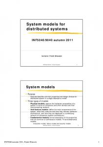
Figure 4: The simplest method to merge new topics in AD-HDP is by integer topic label. single set of globally-consistent word-topic counts . We refer to the distributed version of HDP as AD-HDP, and provide the pseudocode in Algorithm 3. Unlike AD-LDA, which uses a fixed number of topics, individual processors in AD-HDP may instantiate new topics during the sampling phase, according to the HDP sampling equation (5). During the synchronization and update step, instead of treating each processor’s new topics as distinct, we merge new topics that were instantiated on different processors. Merging new topics helps limit unnecessary growth in the total number of topics and allows AD-HDP to produce more of a global model. There are several ways to merge newly created topics on each processor. A simple way – inspired by AD-LDA – is to merge new topics based on their integer topic label. A more complicated way is to match new topics across processors based on topic similarity. In the first merging scheme, new topics are merged based on their integer topic label. For example, assume that we have three processors, and at the end of a sweep through the data, processor one has 8 new topics, processor two has 6 new topics, and processor three has 7 new topics. Then during synchronization, all these new topics would be aligned by topic label and their counts summed, producing 8 new global topics, as shown in Figure 4. While this merging of new topics by topic-id may seem suboptimal, it is computationally simple and efficient. We will show in the next section that this merging generally works well in practice, even when processors only have a small amount of data. We suggest that even if the merging by 9


Algorithm 4 Greedy Matching of New Topics for AD-HDP Initialize global set of new topics, , to be processor 1’s set of new topics for = 2 to P do for topic in processor p’s set of new topics do Initialize score array for topic in do score[ ] = symmetric-KL-divergence( , ) end for if min(score) threshold then Add ’s counts to the topic in corresponding to min(score) else Augment with the new topic end if end for end for

topic-id is initially quite random, the subsequent dynamics align the topics in a sensible manner. We will also show that AD-HDP ultimately learns models with similar perplexity to HDP, irrespective of how new topics are merged. We also investigate more complicated schemes for merging new topics in AD-HDP, beyond the simple approach of merging by topic-id. Instead of aligning new topics based topic-id it is possible to align new topics using a similarity metric such as symmetric Kullback-Leibler divergence. However, finding the optimal matching of topics in the case where is NP-hard (Burkard and C ¸ ela, 1999). Thus, we consider approximate schemes: bipartite matching using a reference processor, and greedy matching. In the bipartite matching scheme, we select a reference processor and perform bipartite matching between every processor’s new topics and the set of new topics of the reference processor. The bipartite match is computed using the Hungarian algorithm, which runs in , producing an overall complexity of where is the maximum number of new topics on a processor. We implemented this scheme but did not find any improvement over AD-HDP with merging by topic-id. In the greedy matching scheme, new topics on each processor are sequentially compared to a global set of new topics. This global set is initialized to the first processor’s set of new topics. If a new topic is sufficiently different from every topic in the global set, the number of topics in the global set is incremented; otherwise, the counts for that new topic are added to those from the closest match in the global set. A threshold is used to determine whether a new topic is sufficiently different from another topic. The worst case complexity of this algorithm is – this is the case where every new topic is found to be different from every other new topic in the global set. Increasing this threshold will make it more likely for new topics to merge with the topics already in the global set (instead of incrementing the set), causing the expected running time of this merging algorithm to be linear in the number of processors. The pseudocode of this greedy matching scheme is shown in Algorithm 4. This algorithm is run after each iteration of AD-HDP to produce a global set of new topics. We show in the next section that this greedy matching scheme significantly improves the rate of convergence for AD-HDP. 10


train

test

KOS 3,000 6,906 467,714 430

NIPS 1,500 12,419 2,166,058 184

FOR

WIKIPEDIA 2,051,929 120,927 344,941,756 -

T OPIC M ODELS

PUBMED 8,200,000 141,043 737,869,083 -

NEWSGROUPS 19500 27,059 2,057,207 498

Table 2: Characteristics of data sets used in experiments.

4. Experiments The purpose of our experiments is to investigate how our distributed topic model algorithms, ADLDA, HD-LDA and AD-HDP, perform when compared to their sequential counterparts, LDA and HDP. We are interested in two aspects of performance: the quality of the model learned, measured by log probability of test data; and the time taken to learn the model. Our primary data sets for these experiments were KOS blog entries, from dailykos.com, and NIPS papers, from books.nips.cc. We chose these relatively small data sets to allow us to perform a large number of experiments. Both data sets were split into a training set and a test set. Size parameters for these data sets are is the number of documents, is the vocabulary size shown in Table 2. For each corpus, and is the total number of words. Two larger data sets WIKIPEDIA, from en.wikipedia.org, and PUBMED, from pubmed.gov were used for speedup experiments, described in Section 5. For precision-recall experiments we used the NEWSGROUPS data set, taken from the UCI Machine Learning Repository. All the data sets used in this paper can be downloaded from the UCI Machine Learning Repository (Asuncion and Newman, 2007). Using the KOS and NIPS data sets, we computed test set perplexities for a range of topics , and for numbers of processors, , ranging from 1 to 3000. The distributed algorithms were initialized by first randomly assigning topics to words in , then counting topics in documents, , and words in topics, , for each processor. For each run of LDA, AD-LDA, and HD-LDA, a sample was taken at 500 iterations of the Gibbs sampler, which is well after the typical burn-in period of the initial 200-300 iterations. For each run of HDP and AD-HDP, we allow the Gibbs sampler to run for 3000 iterations, to allow the number of topics to grow. In our perplexity experiments, multiple processors were simulated in software by separating data, running sequentially through each processor, and simulating the global synchronization and update steps. For the speedup experiments, computations were run on 64 to 1024 processors on a 2000+ processor parallel supercomputer. The following set of hyperparameters was used for the experiments, where hyperparameters are shown as variables in squares in the graphical models in Figures 1 and 3. For AD-LDA we set and . For AD-HDP we set , Gamma and Gamma . While and could have also been fixed, resampling these hyperparameters allows for more robust topic growth, as described by Teh et al. (2006). For LDA and AD-LDA we fixed the hyperparameters and , but these priors could also be learned using sampling. Selection of hyperparameters for HD-LDA was guided by our experience with AD-LDA. For AD-LDA, , but for HD-LDA , so we choose and to make the mode of to simulate the inclusion of global counts in as is done in AD-LDA. We set , because it is important to scale by the number of topics to prevent oversmoothing when the counts are spread thinly among many topics. Finally, we choose and to make the mode 11


of set:

, matching the value of used in our LDA and AD-LDA experiments. Specifically, we , , and . To systematically evaluate our distributed topic model algorithms, AD-LDA, HD-LDA and AD-HDP, we measured performance using test set perplexity, which is computed as Perp test test . For every test document, half the words at random are designated for foldtest in, and the remaining words are used as test. The document mixture is learned using the fold-in part, and log probability of the test words is computed using this mixture, ensuring that the test words are not used in estimation of model parameters. For AD-LDA, the perplexity computation exactly follows that of LDA, since a single set of topic counts are saved when a sample is taken. In contrast, all copies of are required to compute perplexity for HD-LDA. Except where stated, perplexities are computed for all algorithms using samples from the posterior from ten independent chains using test

test

(9)

This perplexity computation follows the standard practice of averaging over multiple chains when making predictions with LDA models trained via Gibbs sampling, as discussed in Griffiths and Steyvers (2004). Averaging over ten samples significantly reduces perplexity compared to using a single sample from one chain. While we perform averaging over multiple samples to improve the estimate of perplexity, we have also observed similar relative results across our algorithms when we use a single sample to compute perplexity. Analogous perplexity calculations are used for HD-LDA and AD-HDP. With HD-LDA we additionally compute processor-specific responsibilities, since test documents do not belong to any particular processor, unlike the training documents. Each processor learns a document mixture using the fold-in part for each test document. For each processor, the likelihood is calculated over the words in the fold-in part in a manner analogous to (9), and these likelihoods are normalized to form the responsibilities, . To compute perplexity, we compute the likelihood over the test words, using a responsibility-weighted average of probabilities over all processors: test

test

(10)

where Computing perplexity in this manner prevents the possibility of seeing or using test words during the training and fold-in phases. 4.1 Perplexity The perplexity results for KOS and NIPS in Figure 5 clearly show that the model perplexity is essentially the same for the distributed models AD-LDA and AD-HDP at and as their single-processor versions at . The figures show the test set perplexity, versus number of processors, , for different numbers of topics for the LDA-type models, and also for the HDPmodels which learn the number of topics. The perplexity is computed by LDA (circles) and HDP (triangles), and we use our distributed algorithms – AD-LDA (crosses), HD-LDA (squares), 12


FOR

T OPIC M ODELS

and AD-HDP (stars) – to compute the and perplexities. The variability in perplexity as a function of the number of topics is much greater than the variability due to the number of processors. Note that there is essentially no perplexity difference between AD-LDA and HD-LDA. KOS Data Set

1800 K=8

1900

1700

1500 1400

K=10

1800 1700

K=16 LDA AD−LDA HD−LDA HDP AD−HDP

Perplexity

Perplexity

1600

NIPS Data Set

2000

K=32

1600

LDA AD−LDA HD−LDA HDP AD−HDP

K=40

1500 1400

K=64

K=20

K=80

1300

1300

1200

HDP

1200

P=1

P=10 Number of Processors

1100

P=100

HDP

P=1

P=10 Number of Processors

P=100

Figure 5: Test perplexity on KOS (left) and NIPS (right) data versus number of processors P. corresponds to LDA and HDP. At and we show AD-LDA, HD-LDA and AD-HDP.

KOS Data Set

1750

NIPS Data Set

2000

T=8

1700

T=10

1900 1800

1600

T=16

Perplexity

Perplexity

1650

1550 1500

T=20

1700 1600

T=32

T=40

1450 1500

1400 1350 0 10

T=64 1

10

2

3

10 10 Number of processors P

4

10

1400 0 10

T=80 1

10

2

3

10 10 Number of processors P

4

10

Figure 6: AD-LDA test perplexity versus number of processors up to the limiting case of number of processors equal to number of documents in collection. Left plot shows perplexity for KOS and right plot shows perplexity for NIPS.

13


Even in the limit of a large number of processors, the perplexity for the distributed algorithms matches that for the sequential version. In fact, in the limiting case of just one document per processor, for KOS and for NIPS, we see that the perplexities of AD-LDA are generally no different to those of LDA, as shown in the rightmost point in each curve in Figure 6. AD-HDP instantiates fewer topics but produces a similar perplexity to HDP. The average number of topics instantiated by HDP on KOS was 669 while the average number of topics instantiated by AD-HDP was 490 ( ) and 471 ( ). For NIPS, HDP instantiated 687 topics while AD-HDP instantiated 569 ( ) and 569 ( ) topics. AD-HDP instantiates fewer topics because of the merging across processors of newly-created topics. The similar perplexity results for AD-HDP compared to HDP, despite the fewer topics, is partly due to the relatively small probability mass in many of the topics. Despite no formal convergence guarantees, the approximate distributed algorithms, AD-LDA and AD-HDP, converged to good solutions in every single experiment (of the more than one hundred) we conducted using multiple real-world data sets. We also tested both our distributed LDA algorithms with adversarial/non-random distributions of topics across processors using synthesized data. One example of an adversarial distribution of documents is where each document only uses a single topic, and these documents are distributed such that processor only has documents that are about topic . In this case the distributed topic models have to learn the correct set of topics, even though each processor only sees local documents that pertain to just one of the topics. We ran multitopics (i.e. each ple experiments, starting with 1000 documents that were hard-assigned to document is only about one topic), and distributing the 1000 documents over processors, where each processor contained documents belonging to the same topic (an analogy is one processor only having documents about sports, the next processor only having documents about arts, and so on). The perplexity performance of AD-LDA and HD-LDA under these adversarial/non-random distribution of documents was as good as the performance when the documents were distributed randomly, and as good as the performance of single-processor LDA. To demonstrate that the low perplexities obtained from the distributed algorithms with processors are not just due to averaging effects, we split the NIPS corpus into one hundred 15-document collections, and ran LDA separately on each of these hundred collections. The test perplexity at computed by averaging 100-separate LDA models was 2117, significantly higher than the test perplexity of 1575 for AD-LDA and HD-LDA. This shows that a baseline approach of simple averaging of results from separate processors performs much worse than the distributed coordinated learning algorithms that we propose in this paper. 4.2 Convergence One could imagine that distributed algorithms, where each processor only sees its own local data, may converge more slowly than single-processor algorithms where the data is global. Consequently, we performed experiments to see whether our distributed algorithms were converging at the same rate as their sequential counterparts. If the distributed algorithms were converging slower, the computational gains of parallelization would be reduced. Our experiments consistently showed that the convergence rate for the distributed LDA algorithms was just as fast as those for the single processor case. As an example, Figure 7 shows test perplexity versus iteration of the Gibbs sampler for the NIPS data at topics. During burn-in, up to iteration 200, the distributed algorithms are actually converging slightly faster than single processor LDA. Note that one iteration of AD-LDA or 14


FOR

T OPIC M ODELS

HD-LDA on a parallel multi-processor computer only takes a fraction (at best time of one iteration of LDA on a single processor computer. LDA AD−LDA P=10 AD−LDA P=100 HD−LDA P=10 HD−LDA P=100

2200 2100

Perplexity

) of the wall-clock

2000 1900 1800 1700 50

100

150

200 250 Iteration

300

350

400

Figure 7: Convergence of test perplexity versus iteration for the distributed algorithms AD-LDA and HD-LDA using the NIPS data set and topics.

We see slightly different convergence behavior in the non-parametric topic models. AD-HDP converges more slowly than HDP, as shown in Figure 8, due to AD-HDP’s heavy averaging of new topics resulting from merging by topic-id (i.e. no matching). This slower convergence may partially be a result of the lower number of topics instantiated. The number of new topics instantiated in one pass of AD-HDP is limited to the maximum number of new topics instantiated on any one processor. For example, in the right plot, after 500 iterations, HDP has instantiated 360 topics, whereas ADHDP has instantiated 210 ( ) and 250 ( ) topics. Correspondingly, at 500 iterations, the perplexity of HDP is lower than the perplexity of AD-HDP. After three thousand iterations, ADHDP produces the same perplexity as HDP, which is reassuring because it indicates that AD-HDP is ultimately producing a model that has the same predictive ability as HDP. We observe a similar result for the NIPS data set. One way to accelerate the rate of convergence for AD-HDP is to match newly generated topics by similarity instead of by topic-id. Figure 9 shows that performing the greedy matching scheme for new topics as described in Algorithm 4 significantly improves the rate of convergence for AD-HDP. In this experiment, we used a threshold of 2 for determining topic similarity. The number of topics increases at a faster rate for AD-HDP with matching, since the greedy matching scheme is more flexible in that the number of new topics at each iteration is not limited to the maximum number of new topics instantiated on any one processor. The results show that the greedy matching scheme enables AD-HDP to converge almost as quickly as HDP. In practice, only a few new topics are generated locally on each processor each iteration, and so the computational overhead of this heuristic matching scheme is minimal relative to the time for Gibbs sampling. 15


1800

1000

HDP AD−HDP P=10 AD−HDP P=100

1700

900 800 Number of Topics

Perplexity

1600 1500 1400

700 600 500 400 300 200

1300

HDP AD−HDP P=10 AD−HDP P=100

100 1200 0

500

1000

1500 Iteration

2000

2500

0 0

3000

500

1000

1500 Iteration

2000

2500

3000

Figure 8: Results for HDP versus AD-HDP with no matching. Left plot shows test perplexity versus iteration for HDP and AD-HDP. Right plot shows number of topics versus iteration for HDP and AD-HDP. Results are for the KOS data set. 1800

1000

HDP AD−HDP P=100 AD−HDP P=100 (with matching)

1700


Perplexity

1600 1500 1400

700 600 500 400 300 200

1300

HDP AD−HDP P=100 AD−HDP P=100 (with matching)

100 1200 0

500

1000

1500 Iteration

2000

2500

3000

0 0

500

1000

1500 Iteration

2000

2500

3000

Figure 9: Results for HDP versus AD-HDP with greedy matching. Left plot shows test perplexity versus iteration for HDP and AD-HDP. Right plot shows number of topics versus iteration for HDP and AD-HDP. Results are for the KOS data set.

To further check that the distributed algorithms were performing comparably to their single processor counterparts, we ran experiments to investigate whether the results were sensitive to the number of topics used in the models, in case the distributed algorithms’ performance worsens when the number of topics becomes very large. Figure 10 shows the test perplexity computed on the NIPS data set, as a function of the number of topics, for the LDA algorithms and a fixed number of processors (the results for the KOS data set were quite similar and therefore not shown). The perplexities of the different algorithms closely track each other as number of topics, , increases. In fact, in some cases HD-LDA produces slightly lower perplexities than those of single processor 16


FOR

T OPIC M ODELS

LDA. This lower perplexity may be due to the fact that in HD-LDA test perplexity is computed using P sets of topic parameters, thus it has more parameters than AD-LDA to better fit the data. 2000

LDA AD−LDA P=10 HD−LDA P=10

1900 1800

Perplexity

1700 1600 1500 1400 1300 1200 1100 1000 0

100

200


500

600

700

Figure 10: Test perplexity versus number of topics using the NIPS data set (S=5).

4.3 Precision and Recall In addition to our experiments measuring perplexity, we also performed precision/recall calculations using the NEWSGROUPS data set, where each document’s corresponding newsgroup is the class label. In this experiment we use LDA and AD-LDA to learn topic models on the training data. Once the model is learned, each test document can be treated as a ”query”, where the goal is to retrieve relevant documents from the training set. For each test document, the training documents are ranked according to how probable the test document is under each training document’s mixture and the set of topics . From this ranking, one can calculate mean average precision and area under the ROC curve. 0.9

0.16

0.85 Mean Area Under ROC Curve

Mean Average Precision

0.14 0.12 0.1 0.08 0.06 0.04 0

LDA AD−LDA P=10 AD−LDA P=100 10

20

Iteration

30

40

0.8 0.75 0.7 0.65 0.6 LDA AD−LDA P=10 AD−LDA P=100

0.55 50

0.5 0

10

20

Iteration

30

40

50

Figure 11: Precision/recall results: (left) Mean average precision for LDA/AD-LDA. (right) Area under the ROC curve for LDA/AD-LDA.

17


Figure 11 shows the mean average precision and the area under the ROC curve achieved by LDA and AD-LDA, plotted versus iteration. LDA performs slightly better than AD-LDA for the first 20 iterations, but AD-LDA catches up and converges to the same mean average precision and area under the ROC curve as LDA. This again shows that our distributed/parallel version of LDA produces a very similar result to the single-processor version.

5. Scalability The primary motivation for developing distributed algorithms for LDA and HDP is to have highly scalable algorithms, in terms of memory and computation time. Memory requirements depend on both memory for data and memory for model parameters. The memory for the data scales with , the total number of words in the corpus. The memory for the parameters is linear in the number of topics , which is either fixed for the LDA models or learned for the HDP models. The perprocessor per-iteration time and space complexity of LDA and AD-LDA are shown in Table 3. AD-LDA’s memory requirement scales well as collection sizes grow, because while corpus size ( and ) can get arbitrarily large, which can be offset by increasing the number of processors, , the vocabulary size will tend to asymptote, or at least grow more slowly. Similarly the time complexity scales well since the leading order term is divided by . The communication cost of the reduce operation, denoted by in the table, represents the time taken to perform the global sum of the count difference . This is executed in stages and can be implemented efficiently in standard language/protocols such as MPI, the Message Passing Interface. Because of the additional term, parallel efficiency will depend on , with increasing efficiency as this ratio increases. Space and time complexity of HD-LDA are similar to that of AD-LDA, but HD-LDA has bigger constants. For a given number of topics, , we argue that AD-HDP has similar time complexity as AD-LDA. We performed large-scale speedup experiments with just AD-LDA instead of all three of our distributed topic modeling algorithms because AD-LDA produces very similar results to HD-LDA, but with significantly less computation. We expect that relative speedup performance for HD-LDA and AD-HDP should follow that for AD-LDA. LDA

AD-LDA

Space Time Table 3: Space and time complexity of LDA and AD-LDA.

We used two multi-million document data sets, WIKIPEDIA and PUBMED, for speedup experiments on a large-scale supercomputer. The supercomputer used was DataStar, a 15.6 TFlop terascale machine at San Diego Supercomputer Center built from 265 IBM P655 8-way compute nodes. We implemented a parallel version of AD-LDA using the Message Passing Interface protocol. We ran AD-LDA on WIKIPEDIA using topics and PUBMED using topics distributed over and 1024 processors. The speedup results, shown in Figure 12, show relatively high parallel efficiency, with approximately 700 times speedup for WIKIPEDIA and 800 times speedup for PUBMED when using processors, corresponding to parallel efficiencies of approximately 0.7 and 0.8 respectively. This speedup is computed relative to the 18


1000 900

FOR

T OPIC M ODELS

Perfect AD−LDA (PUBMED) AD−LDA (WIKIPEDIA)

800

Speedup

700 600 500 400 300 200 100 0 0

200

400 600 Number of processors

800

1000

Figure 12: Parallel speedup results for 64 to 1024 processors on multi-million document datasets WIKIPEDIA and PUBMED.

time per iteration when using processors (i.e. at processors speedup=64), since it is not possible, due to memory limitations, to run these models on a single processor. Multiple runs were timed for both WIKIPEDIA and PUBMED, and the resulting variation in timing was less than 1%, so error bars are not shown in the figure. We see slightly higher parallel efficiency for PUBMED versus WIKIPEDIA because PUBMED has a larger amount of computation per unit data communicated, . This speedup dramatically reduces the learning time for large topic models. If we were to learn a topic model for PUBMED using LDA on a single processor, it would require over 300 days instead of the 10 hours required to learn the same model using AD-LDA on 1024 processors. In our speedup experiments on these large data sets, we did not directly investigate latency or communication bandwidth effects. Nevertheless, one could expect that if the communication time becomes very long compared to the computation time, then it may be worth doing multiple Gibbs sampling sweeps on a processor’s local data before performing the synchronization and global update step. In Section 6 we further examine this question of frequency of synchronizations. The relative time for communication versus computation also effects the weak scaling of parallelization, where the problem size increases linearly with the number of processors. We expect that parallel efficiency will be relatively constant for weak scaling since is constant. In addition to the large-scale speedup experiments run on the 1024-processor parallel supercomputer, we also performed small-scale speedup experiments for AD-HDP on an 8-node parallel cluster running MPI. Using the NIPS data set we measured parallel efficiencies of 0.75 and 0.5 for and . The latter result on 8 processors means that the HDP model for NIPS can be learned four times faster than on a single processor. 19


6. Analysis of Approximate Distributed LDA Finally, we investigate the dynamics of AD-LDA learning using toy data to get further insight into how AD-LDA is working. While we have shown experimental results showing that AD-LDA produces models with similar perplexity and similar convergence rates to LDA, it is not obvious words and why this algorithm works so well in practice. Our toy example has topics. We generated document collections according to the LDA generative process given by (1). We chose a low dimension vocabulary, , so that we could plot the evolution of the Gibbs sampler on a two-dimensional word-topic simplex. We first generated data, then learned models using LDA and AD-LDA. The left plot of Figure 13 shows the distance between the model’s estimate of a particular topic-word distribution and the true distribution, as a function of Gibbs iteration, for both singleprocessor LDA and AD-LDA with . LDA and AD-LDA have qualitatively the same threephase learning dynamics. The first four or so iterations (labeled initialize) correspond to somewhat random movement close to the randomly initialized starting point. In the next phase (labeled burnin) both algorithms rapidly move in parameter space toward the posterior mode. And finally after burn-in (labeled stationary) both are sampling around the mode. In the right plot we show the similarity between AD-LDA and LDA samples taken from the equilibrium distribution – here plotted on the two-dimensional planar simplex corresponding to the three-word topic distribution. 0.4 0.35

LDA AD−LDA proc1 AD−LDA proc2

initialize

L1 norm

0.3

0.475

0.25 0.2

0.465 burn−in

0.46

0.15

0.455

0.1

0.45

0.05 0 0

topic mode

0.47

stationary 20

40

Iteration

LDA AD−LDA

0.445 60

80

100 0.8

0.81

0.82

0.83

0.84

0.85

Figure 13: (Left) distance to the mode for LDA and for AD-LDA. (Right) Closeup of 50 samples of (projected onto the topic simplex) taken from the equilibrium distribution, showing the similarity between LDA and AD-LDA. Note the zoomed scale in this figure. The left plot of Figure 14 depicts the same trajectory shown in Figure 13 left, projected onto the topic simplex. This plot shows the paths in parameter space of each model, and the same three-phase learning dynamics: taking a few small steps near the starting point, moving up to the true solution, and then sampling near the posterior mode for the rest of the iterations. For each Gibbs iteration, the parameters corresponding to each of the two individual processors, and those parameters after merging, are shown for AD-LDA. One can see the alternating pattern of two separate (but close) 20


FOR

T OPIC M ODELS

parameter estimates on each processor, followed by a merged estimate. We observed that after the initial few iterations, the individual processor steps and the merge step each resulted in a move closer to the mode. One might worry that the AD-LDA algorithm would get trapped close to the initial starting point, e.g., due to repeated label switching or oscillatory behavior of topic labeling across processors. In practice we have consistently observed that the algorithm quickly discards such configurations due to the stochastic nature of the moves and latches onto a consistent and stable labeling that rapidly moves it toward the posterior mode. The figure clearly illustrates that LDA and AD-LDA have qualitatively similar learning dynamics. The right plot in Figure 14 illustrates the same qualitative behavior as in the left plot, but now for processors. Interestingly, across a wide range of experiments, we observed that the variance in the ADLDA word-topic distribution samples is typically only about 70% of the variance in LDA topic samples. Since the samplers are not the same it makes sense that the posterior variance differs (i.e. is underestimated) by the parallel sampler. We expect less variance because AD-LDA ignores fluctuations in the bulk of . Nonetheless, all of our experiments indicate that the posterior mode and means found by the parallel sampler are essentially the same as those found by the sequential sampler. 0.5

0.5

0.48

0.48

0.46

0.46 topic mode

0.44 0.42

0.42

0.4

0.4

0.38

start

0.36 0.65

LDA AD−LDA proc1 AD−LDA proc2 0.7

0.75

0.8

0.85

topic mode

0.44

0.38 0.9

LDA AD−LDA proc1 AD−LDA proc2 AD−LDA proc3 ...etc... AD−LDA proc10

start

0.36 0.65

0.7

0.75

0.8

0.85

Figure 14: (Left) Projection of topics onto simplex, showing convergence to mode for (Right) Same as left plot, but with .

0.9

.

Another insight can be gained by thinking of LDA as an approximation to stochastic descent in the space of assignment variables . On a single processor, one can view Gibbs sampling during burn-in as a stochastic algorithm to move up the likelihood surface. With multiple processors, each processor computes an upward direction in its own subspace, keeping all other directions fixed. The global update step then recombines these directions by vector-addition, in the same way as one would compute a gradient using finite differences. This is expected to be accurate as long as the surface is locally convex or concave, but will break down at saddle-points. We conjecture AD-LDA works reliably because saddle points are unstable and rare because the posterior is usually highly peaked for LDA models and high-dimensional count data sets. While we see similar perplexities for AD-LDA compared to LDA, we could further ask if the AD-LDA algorithm is producing any bias in its estimates of the model parameters. To test this, we 21


0.09 0.08 0.07

||E(φ)−φref||

0.06 0.05

reference = LDA reference = true

0.04 0.03 0.02 0.01 0 0 10

Figure 15: Average

1

10

2

3

10 10 Number of processors, P

4

10

error in word-topic distribution versus P for AD-LDA.

performed a series of experiments where we generated synthetic data sets according to the LDA generative process, with known word-topic distributions . We then learned LDA and AD-LDA models from each of the simulated data sets. We computed the expected value of the AD-LDA topics and compared this to two reference values, ref one based on the true distribution, ref , the other based on multiple LDA samples, ref . Figure 15 shows that AD-LDA is much LDA closer to the LDA topics , telling us that the sampling LDA than either are to the true topics variation in learning LDA models from finite data sets is much greater than the variation between LDA and AD-LDA on the same data sets. When Does AD-LDA Fail? In all of our experiments thus far, we have seen that our distributed algorithms learn models with equivalent predictive power as their non-distributed counterparts. However, when global synchronizations are done less frequently (i.e., when the synchronization step is performed after multiple Gibbs sampling sweeps through local data), the distributed algorithms may converge to suboptimal solutions. When the synchronization interval is increased dramatically, it is possible for AD-LDA to converge to a suboptimal solution. This can happen because the topics (with the same integer label) on each processor can drift far apart, so that topic on one processor diverges from topic on another processor. In Figure 16, we show the results of an experiment on KOS where synchronizations only occur once every 100 iterations. For processors, AD-LDA performs significantly worse than LDA. The processor case is the worst case for AD-LDA, since one half of the total words on each processor have the freedom to drift. In contrast, when processors, each processor can only locally modify 1/100 of the topic assignments, and so the topics on each processor can not drift far from the global set of topic counts at the previous iteration. Bipartite matching significantly 22


FOR

T OPIC M ODELS

improves the perplexity in the processor case, suggesting that the lack of communication has indeed caused the topics to drift apart. Fortunately, topic drifting becomes less of a problem as more processors are used, and can be eliminated by frequent synchronization. It is also important to note that AD-LDA , where processors synchronize after every iteration, gives essentially identical results as LDA. Our recommendation in practice is to perform the synchronization and count updates after each iteration of the Gibbs sampler. As shown earlier in the paper, this leads to performance that is essentially indistinguishable from LDA. Since most multi-processor computing hardware will tend to have communication bandwidth matched to processor speed (i.e. faster and/or more processors usually come with a faster communication network), synchronizing after each iteration of the Gibbs sampler will usually be the optimal strategy. 2500

LDA AD−LDA P=2 AD−LDA P=2, Sync=100 AD−LDA P=2, Sync=100 (with matching) AD−LDA P=100, Sync=100

2400

Perplexity

2300 2200 2100 2000 1900 1800 1700 0

1000

2000 3000 Iteration

4000

5000

Figure 16: Test perplexity versus iteration where synchronizations between processors only occur every 100 iterations, KOS, .

7. Related Work Approximate inference for topic models such as LDA and HDP can be carried out using a variety of methods, the most common being variational methods and Markov chain Monte Carlo methods. Previous efforts to parallelize these algorithms have focused on variational methods, which are often straightforward to cast in a distributed framework. For example, Blei et al. (2002) and Nallapati et al. (2007) describe distributed variational EM methods for LDA. In their distributed variational approach, the computationally expensive E-step is easily parallelized because the document-specific variational parameters are independent. Wolfe et al. (2008) investigate the parallelization of both the E and M-steps of variational EM for LDA, under a variety of computer network topologies. In these cases the distributed version of LDA produces identical results to the sequential version of the algorithm. However, memory for variational inference in LDA scales as , where is the number of distinct document-word pairs in the corpus. For typical English-language corpora, the total number of words in the corpus is less than twice the number of distinct document-word pairs 23


( ), so can be considered on the order of . Since is usually much larger than the number of documents, , this memory requirement of is not nearly as scalable as that the memory requirement of for MCMC methods. Parallelized versions of various machine learning algorithms have also been developed. Forman and Zhang (2000) describe a parallel k-means algorithm, and W. Kowalczyk and N. Vlassis (2005) describe an asynchronous parallel EM algorithm for Gaussian mixture learning. A parallel EM algorithm for Probabilistic Latent Semantic Analysis, implemented using Google’s MapReduce framework, was described in Das et al. (2007). A review of how to parallelize an array of standard machine learning algorithms using MapReduce was presented by Chu et al. (2007). Rossini et al. (2007) presents a framework for statisticians that allows for the parallel computing of independent tasks within the R language. While many of these EM algorithms are readily parallelizable, Gibbs sampling of dependent variables (such as topic assignments) is fundamentally sequential and therefore difficult to parallelize. One way to parallelize Gibbs sampling is to run multiple independent chains in parallel to obtain multiple samples; however, this multiple-chain approach does not address the fact that the burn-in within each chain may take a long time. Furthermore, for some applications, one is not interested in multiple samples from independent chains. For example, if we wish to learn topics for a very large document collection, one is usually satisfied with mean values of word-topic distributions taken from a single chain. One can parallelize a single MCMC chain by decomposing the variables into independent noninteracting blocks that can be sampled concurrently (Kontoghiorghes, 2005). However, when the variables are not independent, sampling variables in parallel is not possible. Brockwell (2006) presents a general parallel MCMC algorithm based on pre-fetching, but it is not practical for learning topic models because it discards most of its computations which makes it relatively inefficient. It is possible to construct partially parallel Gibbs samplers, in which the samples are independently accepted with some probability. In the limit as this probability goes to zero, this sampler will approach the sequential Gibbs sampler, as explained in P. Ferrari et al. (1993). However, this method is also not practical when learning topic models because it is computationally inefficient. Younes (1998) shows the existence of exact parallel samplers that make use of periodic synchronous random fields. However there is no known method for constructing such a sampler. Our HD-LDA model is similar to the DCM-LDA model presented by Mimno and McCallum (2007). There the authors perform topic modeling on a collection of books by learning a different topic model for each book and then clustering these learned topics together to find global topics. In this model, the concept of a book is directly analogous to our concept of a processor. DCM-LDA uses Stochastic EM along with agglomerative clustering to learn topics, while our HD-LDA follows a fully Bayesian approach for inference. HD-LDA also differs from other topic hierarchies found in the literature. The Hierarchical Dirichlet Process model of Teh et al. (2006) places a deeper hierarchical prior on the topic mixture, instead of on the word-topic distributions. The Pachinko Allocation Model presented by Li and McCallum (2006) deals with a document-specific hierarchy of topic-assignments. These types of hierarchies do not directly facilitate proper parallel Gibbs sampling as is done in HD-LDA. 24


FOR

T OPIC M ODELS

8. Conclusions We have proposed three different algorithms for distributing across multiple processors Gibbs sampling for LDA and HDP. With our approximate distributed algorithm, AD-LDA, we sample from an approximation to the posterior distribution by allowing different processors to concurrently sample topic assignments on their local subsets of the data. Despite having no formal convergence guarantees, AD-LDA works very well empirically and is easy to implement. With our hierarchical distributed model, HD-LDA, we adapt the underlying LDA model to map to the distributed processor architecture. This model is more complicated than AD-LDA, but it inherits the usual convergence properties of Markov chain Monte Carlo. We discovered that careful selection of hyperparameters was critical to making HD-LDA work well, but this selection was clearly informed by AD-LDA. Our distributed algorithm AD-HDP followed the same approach as AD-LDA, but with an additional step to merge newly instantiated topics. Our proposed distributed algorithms learn LDA models with predictive performance that is no different than single-processor LDA. On each processor they burn-in and converge at the same rate as LDA, yielding significant speedups in practice. For HDP, our distributed algorithm eventually produced the same perplexity as the single-processor version of HDP. Prior to reaching the converged perplexity result, AD-HDP had higher perplexity than HDP since the merging of new topics by label slows the rate of topic growth. We also discovered that matching new topics by similarity significantly improves AD-HDP’s rate of convergence. The space and time complexity of these distributed algorithms make them scalable to run very large data sets, for example, collections with billions to trillions of words. Using two multi-million document datasets, and running computations on a 1024-processor parallel supercomputer, we showed how one can achieve a 700-800 times reduction in wall-clock time by using our distributed approach. There are several potentially interesting research directions that can be pursued using the algorithms proposed here as a starting point. One research direction is to use more complex schemes that allow data to adaptively move from one processor to another. The distributed schemes presented in this paper can also be used to parallelize topic models that are based on or derived from LDA and HDP, and beyond that a potentially larger class of graphical models.

Acknowledgments This material is based upon work supported by the National Science Foundation. DN and PS were supported by NSF grants SCI-0225642, CNS-0551510, and IIS-0083489. DN was also supported by a Google Research Award. PS was also supported by ONR grant N00014-18-1-101 and a different Google Research Award. AA was supported by an NSF graduate fellowship. MW was supported by NSF grants IIS-0535278 and IIS-0447903, and ONR grant 00014-06-1-073. Computations were performed at SDSC under an MRAC Allocation.

25


Appendix A. The auxiliary variable method explained in Escobar and West (1995) and Teh et al. (2006) is used to sample , , and . To derive Gibbs sampling equations, we use the following expansions: (11) (S is Stirling number of first kind)

(12)

The first expansion follows from the definition of the Beta function, and the second expansion makes use of the Stirling number of the first kind to rewrite the factorial (see (Abramowitz and Stegun, 1964)). Now we derive the sampling equation for . Combining the collapsed distribution (7) with the prior on (6) gives the posterior distribution for 1 :

(13) Using the expansions (11,12) we introduce the auxiliary variables and :

(14) The joint distribution above allows us to create sampling equations for

, , and :

Gamma

(15)

Beta

(16)

Antoniak

(17)

1. To avoid notational clutter, we denote conditioned-upon variables and parameters by a dash. These variables can be inferred from context.

26


FOR

T OPIC M ODELS

The Antoniak distribution is the distribution of the number of occupied tables if customers are sent into a restaurant that follows the Chinese restaurant process with strength parameter . Sampling from the Antoniak distribution is done by sampling Bernoulli variables: Bernoulli

(18) (19)

Using the same auxiliary variable techniques, we derive sampling equations for and . These variables are sampled jointly because they are dependent. The posterior distribution for and and the joint distribution with the auxiliary variables and are given by: (20)

(21) Note that the set of variables ( and ) is unrelated to the set of auxiliary variables introduced for . The sampling equations for , , , and are:

Gamma

(22)

Dirichlet

(23)

Beta

(24)

Antoniak

(25)

27


References M. Abramowitz and I. Stegun. Handbook of Mathematical Functions with Formulas, Graphs, and Mathematical Tables. Dover, New York, 1964. A. Asuncion and D. Newman. UCI machine learning repository, http://www.ics.uci.edu/ mlearn/MLRepository.html.

2007.

URL

D. Blei, A. Ng, and M. Jordan. Latent Dirichlet allocation. In Advances in Neural Information Processing Systems, volume 14, pages 601–608, Cambridge, MA, 2002. MIT Press. D. Blei, A. Ng, and M. Jordan. Latent Dirichlet allocation. Journal of Machine Learning Research, 3:993–1022, 2003. A. Brockwell. Parallel Markov chain Monte Carlo simulation by pre-fetching. Journal of Computational & Graphical Statistics, 15, No. 1:246–261, 2006. R. Burkard and E. C ¸ ela. Linear assignment problems and extensions. In P. Pardalos and D. Du, editors, Handbook of Combinatorial Optimization, Supplement Volume A. Kluwer Academic Publishers, 1999. G. Casella and C. Robert. Rao-Blackwellisation of sampling schemes. Biometrika, 83(1):81–94, 1996. C. Chemudugunta, P. Smyth, and M. Steyvers. Modeling general and specific aspects of documents with a probabilistic topic model. In Advances in Neural Information Processing Systems 19, pages 241–248. MIT Press, Cambridge, MA, 2007. C. Chu, S. Kim, Y. Lin, Y. Yu, G. Bradski, A. Ng, and K. Olukotun. Map-Reduce for machine learning on multicore. In Advances in Neural Information Processing Systems 19, pages 281– 288. MIT Press, Cambridge, MA, 2007. A. Das, M. Datar, A. Garg, and S. Rajaram. Google news personalization: Scalable online collaborative filtering. In WWW ’07: Proceedings of the 16th International Conference on World Wide Web, pages 271–280, New York, NY, 2007. ACM. M. Escobar and M. West. Bayesian density estimation and inference using mixtures. Journal of the American Statistical Association, 90(430):577–588, 1995. G. Forman and B. Zhang. Distributed data clustering can be efficient and exact. In ACM KDD Explorations, volume 2, pages 34–38, New York, NY, 2000. ACM. T. Griffiths and M. Steyvers. Finding scientific topics. In Proceedings of the National Academy of Sciences, volume 101, pages 5228–5235, 2004. E. Kontoghiorghes. Handbook of Parallel Computing and Statistics (Statistics, Textbooks and Monographs). Chapman & Hall / CRC, 2005. W. Li and A. McCallum. Pachinko allocation: DAG-structured mixture models of topic correlations. In Proceedings of the International Conference on Machine Learning, volume 23, pages 577–584, New York, NY, 2006. ACM. 28


FOR

T OPIC M ODELS

J. Liu, W. Wong, and A. Kong. Covariance structure of the Gibbs sampler with applications to the comparisons of estimators and augmentation schemes. Biometrika, 81(1):27–40, 1994. D. Mimno and A. McCallum. Organizing the OCA: Learning faceted subjects from a library of digital books. In JCDL ’07: Proceedings of the 2007 conference on digital libraries, pages 376–385, New York, NY, 2007. ACM. R. Nallapati, W. Cohen, and J. Lafferty. Parallelized variational EM for latent Dirichlet allocation: An experimental evaluation of speed and scalability. In ICDMW ’07: Proceedings of the Seventh IEEE International Conference on Data Mining Workshops, pages 349–354, Washington, DC, 2007. IEEE Computer Society. P. Ferrari, A. Frigessi, and R. Schonmann. Convergence of some partially parallel Gibbs samplers with annealing. In Annals of Applied Probability, volume 3, pages 137–153. 1993. M. Rosen-Zvi, T. Griffiths, M. Steyvers, and P. Smyth. The author-topic model for authors and documents. In Proceedings of the Conference on Uncertainty in Artificial Intelligence, volume 20, pages 487–494, Arlington, VA, 2004. AUAI Press. A. Rossini, L. Tierney, and N. Li. Simple parallel statistical computing in R. Journal of Computational & Graphical Statistics, 16(2):399, 2007. Y. W. Teh, M. Jordan, M. Beal, and D. Blei. Hierarchical Dirichlet processes. Journal of the American Statistical Association, 101(476):1566–1581, 2006. W. Kowalczyk and N. Vlassis. Newscast EM. In Advances in Neural Information Processing Systems 17, pages 713–720. MIT Press, Cambridge, MA, 2005. J. Wolfe, A. Haghighi, and D. Klein. Fully distributed EM for very large datasets. In Proceedings of the International Conference on Machine Learning, pages 1184–1191. ACM, New York, NY, 2008. L. Younes. Synchronous random fields and image restoration. IEEE Transactions on Pattern Analysis and Machine Intelligence, 20(4):380–390, 1998.

29

Distributed Algorithms for Topic Models - UCI

Distributed Algorithms for Topic Models - UCI

Suggest Documents