Dec 7, 2001 - This article addresses the problem of localization of nodes in a wireless ad hoc communication network. It is motivated by the Sensorwebs and ...
Distributed Localization in Wireless Ad Hoc Networks∗ Slobodan N. Simi´c and Shankar Sastry Department of Electrical Engineering and Computer Sciences University of California Berkeley, CA 94720 December 7, 2001
Abstract We present a distributed algorithm for localization of nodes in a discrete model of a random ad hoc communication network. We compute the expected value of the position estimate, AS , and the probability that AS = 1 cell (the perfect estimate). This leads to bounds of the average complexity of the algorithm at each node.
1
Introduction
This article addresses the problem of localization of nodes in a wireless ad hoc communication network. It is motivated by the Sensorwebs and Smart Dust [KKP] projects at UC Berkeley, whose aim is to develop a unified framework for distributed sensor networks. Recent advances in MEMS, computing, and communication technology have fomented the emergence of massively distributed, wireless sensor networks consisting of hundreds or thousands of nodes. Each node is able to sense the environment, perform simple computations, and communicate with its peers or to an external observer. The challenges these networks present are far beyond the reach of the current theory and algorithms. One way of deploying a sensor network is to scatter the nodes throughout some region of interest. This makes the network topology random. Since there is no a priori communication protocol, the network is ad hoc. The first task that has to be solved is to localize the nodes, i.e., to compute their positions in some fixed coordinate system. Since most applications (such as tracking an object moving through the network, environmental monitoring, etc.) depend on a successful localization, it is of great importance to design scalable localization algorithms The first author was partially supported by the NASA grant NAG-2-1039 and the EPRI grant EPRI35352-6089. ∗
1
and provide error estimates that will enable us to choose optimal network parameters before deployment. Due to high long range communication costs and low battery power, it is natural to seek decentralized, distributed algorithms for sensor networks. This means that instead of relaying data to a central location which does all the computing, the nodes process information in a collaborative, distributed way. For instance, they can form computational clusters, based on their distance from each other. The outcome of these distributed, local computations is stored in local memory and can then be, when necessary, relayed to a centralized computing unit. Robustness to node failures is another reason to seek distributed rather than centralized algorithms. This paper is organized as follows. In Section 2, we establish the setting and introduce the basic terminology and notation. In Section 3, we discuss the basic localization procedure used in the algorithm described in Section 4, and provide basic probabilistic error estimates and simulation results. The proofs are supplied in the Appendix. The first author would like to thank Sekhar Tatikonda for reading a preliminary version of the paper and providing useful comments.
2
Preliminaries
In this section we introduce the basic framework, terminology, and notation. We assume that in a square region Q = [0, s] × [0, s], called the region of operations, we randomly scatter N nodes, S1 , . . . , SN , each of which is equipped with an RF transceiver with communication range r > 0. In other words, a node Si can communicate with every node which lies in its communication region, which is the disk with radius r centered at Si . Each node has a unique ID which is a number between 1 and N . The nodes form an ad hoc network N in which there is an edge between Si and Sj if their distance is less than r. We will call this the continuous model. Even though it is a rather simplified model of how the network is formed, we adopt it because it leads to an easier analytical treatment. However, instead of a disk of radius r, the communication range of a node could instead be an annulus (in case a node is able to decide when a nearby node is at a distance greater than some threshold, based, e.g., on signal strength), an angular sector (if a node is equipped, say, with laser transmitters and receivers that can scan through some angle) or an intersection of an annulus and an angular sector. For more information on these types of constraints, please see [Doh00]. We assume that a certain positive number K of nodes know their location in Q, i.e., they are able to compute their position relative to some fixed coordinate system in Q; in practice this can be achieved by equipping K motes with GPS or a priori (meaning before deploying the ad hoc network) placing in Q a certain number of beacons which can serve to compute the position of the nodes which are within certain distance from them. We call nodes that know their position known nodes and all other ones, unknown nodes. Furthermore, each node has communication as well as sensing capabilities [KKP]. The problems we address in this paper are:
2
• Design a distributed algorithm for localization of nodes in N . • Estimate the complexity and error of the above algorithm. • Find an optimal number of known nodes depending on Q, N , and r, which minimizes the error of the algorithm. Centralized algorithms for localization were studied in [Doh00, DPG00]. The reason we are interested in a distributed rather than a centralized solution is that we envision a massively distributed network in which communication with a centralized computer is expensive both because the power supply of each node is very limited and long-range multi-hop data transmission is costly and often inefficient. However, one quickly discovers that obtaining analytical estimates even in this simple setting can be rather challenging. Furthermore, in the design of a decentralized algorithm relying on node-based data processing, one must take into account that nodes have very limited computational power. This motivates the following discrete approach to the above problems. Let n > 0 be an integer. Partition Q into n2 congruent squares called cells of area (s/n)2 and suppose that for every known node S, we are only interested in finding the cell which contains S. To make this problem tractable, we make a simplifying assumption that the communication range is ρ cells in the max metric, defined by dist ∞ ((i, j), (i0 , j 0 )) = max(|i − i0 |, |j − j 0 |). It is possible for several nodes to lie in the same cell. We call this the discrete model of the network. For example, we can take � � nr ρ= √ , (1) s 2 where [x] denotes the integer part of x. This means that each node S can communicate with every node lying in the square centered at S and containing (2ρ + 1)2 cells. Since all our results are independent of the choice of ρ as a function of r and n, we can clearly select a different value for it. The situation where r is fixed and s, n → ∞ corresponds to increasing the size of the region of operations, while the situation where r/n and s stay constant while n → ∞ corresponds to refining the position estimate. We usually think of n as large and r as much smaller than n. In particular, 2ρ + 1 < n. The last question posed above can now be reformulated in the discrete model as: • Find an optimal number of known nodes, depending on n and ρ, which minimizes the error of the algorithm. It still remains to define what we mean by “the error” of an algorithm, i.e., to define the “metric” by which we measure the accuracy of the algorithm. We will do this in the following section.
3
Q
S1 S2
S PSfrag replacements
S3
Figure 1: Discrete model. Filled circles denote unknown nodes. The dashed line bounds the communication range of the node at its center, with ρ = 3.
3
Localization procedure and error estimates
We now describe the underlying procedure for localization of nodes which can be implemented in both centralized and distributed setting. A distributed implementation is given in the following section. Let S be a random node whose position is unknown. Let Sk1 , . . . , Skm , for some m > 0, be its neighbors in the network N whose positions are known. Two nodes S1 , S2 are neighbors if dist∞ (S1 , S2 ) ≤ ρ. We assume that each Ski knows in which cell it lies, i.e., it is aware of a pair of numbers (xi , yi ), where xi , yi ∈ {1, 2, . . . , n}. We will now use the following notation. For integers 1 ≤ a < b ≤ n, 1 ≤ c < d ≤ n, the “rectangle” [a, b] × [c, d] will denote the union of all cells with grid coordinates (i, j), where a ≤ i ≤ b and c ≤ j ≤ d. Let Bi = [xi − ρ, xi + ρ] × [yi − ρ, yi + ρ]. (2) This is the (discrete) communication region of Ski . Then S ∈ Bi , for all 1 ≤ i ≤ m and therefore m \ S ∈Q∩ Bi . i=1
It is easy to see that
Bi ∩ Bj = [max(xi , xj ) − ρ, min(xi , xj ) + ρ] × [max(yi , yj ) − ρ, min(yi , yj ) + ρ]. 4
This simple formula is, in fact, the main technical reason we choose to work in this discrete setting: one needs much less computing power to calculate the intersection of two squares (with sides parallel to coordinate axes) than to compute the intersection of two discs – only the operations of addition, subtraction, min and max are needed. Thus S ∈ Q ∩ [x+ − ρ, x− + ρ] × [y+ − ρ, y− + ρ],
where x+ = max(x1 , . . . , xm ) and x− = min(x1 , . . . , xm ), and similarly for yi ’s. Finally, since Q = [1, n] × [1, n], we obtain the estimate of the position of S: S ∈ [max(x+ − ρ, 1), min(x− + ρ, n)] × [max(y+ − ρ, 1), min(y− + ρ, n)].
(3)
On the highest level of abstraction we now have the following algorithm (implementable in both centralized and distributed setting) for each unknown node S: Step A Gather the information about the positions of the known neighbors of S. Step B Compute an estimate of the position of S via (3). Let AS be the number of cells in the rectangle on the right hand side of (3), i.e., AS = {min(x− + ρ, n) − max(x+ − ρ, 1) + 1}{min(y− + ρ, n) − max(y+ − ρ, 1) + 1}.
(4)
Let K denote the total number of nodes which know their own position. We will assume that K is given and fixed; later on, we discuss how we can deterministically or randomly generate a sufficiently large number of known nodes. We assume that the position of each node is random and uniformly distributed in [1, n] × [1, n]. Then AS is a random variable with value between 1 and n2 . In the remainder of this section we address the following questions about AS : • What is the expectation E(AS ) of AS ? • What is the probability that AS = 1 cell, i.e., that the estimate is perfect? Having answered these questions, we turn to minimizing |E(AS ) − 1| and maximizing P (AS = 1) as functions of K to find the optimal value for K. Denote by Qρ the square consisting of cells in Q which are at distance ≥ ρ from the boundary. That is, Qρ = [ρ + 1, n − ρ]2 . Then we claim: Theorem 3.1 Let S be a node randomly picked from Qρ . The expectation of AS is �K 2ρ 2ρ+1 � X X (2ρ + 1)2 − kl E(AS ) = 1 + 4 1− . n2 k=1 l=1
Therefore, with n, ρ fixed,
lim E(AS ) = 1,
K→∞
that is, the expectation of the size of the estimate tends to one, the perfect estimate, as the number of known nodes tends to infinity. 5
The proof is provided in the Appendix. Observe that Qρ occupies most of Q, since we assume that ρ is much smaller than n. Given � > 0 and S ∈ Qρ , let K� = K� (n, ρ) be the minimum of all numbers K0 such that |E(AS ) − 1| < �,
(5)
for all K ≥ K0 . Then Corollary 3.1.1 The minimal density of known nodes necessary to achieve (5) satisfies log[8ρ(2ρ + 1)] − log � K� (n, ρ) ≤ . 2 n 2ρ + 1
(6)
Proof: Consider the estimate in Theorem 3.1. Its right hand side is largest when k = 2ρ and l = 2ρ + 1, so � �K 2ρ + 1 . E(AS ) ≤ 1 + 8ρ(2ρ + 1) 1 − n2 Therefore, E(AS ) − 1 < � if
K>
− log[8ρ(2ρ + 1)] + log � � . log 1 − 2ρ+1 n2
(7)
Thus K� is less than or equal to the right hand side of (7). Using the fact that log(1 + x) ≤ x (x > −1), we obtain that K� (n, ρ) ≤ n2
log[8ρ(2ρ + 1)] − log � , 2ρ + 1
as claimed. We denote the right hand side of (6) by δ� (ρ) and interpret it as the critical density of known nodes necessary for the expectation of the estimate to be �-close to the perfect estimate. Denote by HS the number of known neighbors of S. Theorem 3.2 Suppose that S ∈ Qρ . (a) The conditional probability that AS = 1 given that HS = m is � � �m � 4 2ρ P (AS = 1|HS = m) = 1 − . n (b) The probability that AS = 1 is P (AS = 1) =
K � � X K
m=0
m
m K−m
p q
where p = (2ρ + 1)2 /n2 and q = 1 − p. 6
� � �m � 4 2ρ , 1− n
Figure 2: Probability that AS = 1 as a function of ρ and K. Note that P (AS = 1) depends on n, ρ, and K. Its graph for n = 50 is given above (Fig. 2). Corollary 3.2.1 We have "
P (AS = 1) ≥ 1 −
�
2ρ n
� K #4
.
Therefore, P (AS = 1) → 1, as K → ∞. Given p∗ ∈ (0, 1), P (AS = 1) > p∗ if 1/4
log(1 − p∗ )−1 K> . log(n/2ρ) There are several ways of generating nodes with known positions. One is to equip a certain number of nodes with GPS. Another is to a priori place in Q a certain number of beacons whose positions are known. They can be equipped with some relatively sophisticated device capable of localizing objects which lie at a distance ≤ R meters away. Then, if a node lands within R meters from a beacon, its position will be known to that beacon and can be communicated to the node. Suppose that in the latter scenario, the beacons are capable of exactly localizing any node in a region of area α|Q|, for some 0 < α < 1. Then it is not difficult to see that if N nodes are randomly scattered in Q (assuming uniform distribution), the expected value of K will be E(K) = N α. Furthermore,
7
Proposition 3.1 Assuming that K is fixed and given and that S is an unknown node, the expectation of HS is K E(HS ) = 4 [n + ρ(2n − ρ − 1)]2 . n Proof: Let the coordinates of S be (x, y). The communication region of S is B(x, y) = [x − ρ, x + ρ] × [y − ρ, y + ρ] ∩ Q = [max(x − ρ, 1), min(x + ρ, n)] × [max(y − ρ, 1), min(y + ρ, n)]. Denote by p(x, y) the probability that a node lands in the communication region of S = (x, y). It is easy to see that p(x, y) = |B(x, y)|/|Q|, where |B(x, y)| denotes the number of cells in �B(x, y). Set q(x, y) = 1 − p(x, y). The probability that HS = m given S = (x, y) is K p(x, y)m q(x, y)K−m . By a standard calculation in elementary probability it then follows m that E(HS |S = (x, y)) = Kp(x, y). Therefore, by Lemma 6.1(a), E(HS ) = E(E(HS |S = (x, y))) X = E(HS |S = (x, y))P (S = (x, y)) =
(x,y)∈Q n X n X
1 n2
K = n4
Kp(x, y)
x=1 y=1
( n X x=1
[min(x + ρ, n) − max(x − ρ, 1) + 1]
)2
.
Since n X
n−ρ−1
min(x + ρ, n) =
X
(x + ρ) +
x=1
x=1
=
n X
n
x=n−ρ
(n − ρ − 1)(n + ρ) + 2n(ρ + 1) 2
and n X x=1
max(x − ρ, 1) =
ρ+1 X
1+
x=1
= n+ we obtain that
Pn
x=1 [min(x + ρ, n) − max(x − ρ, 1)]
8
n X
x=ρ+2
(x − ρ)
(n − ρ − 1)(n − ρ) , 2 = (2n − ρ − 1)ρ. This completes the proof.
4
Distributed algorithm for localization
In this section we present a simple distributed algorithm for localization, based on the ideas in the previous section. Let S be an arbitrary unknown node in N . The localization algorithm LOCS at S then goes as follows. Step 1 INITIALIZE the estimate: LS = Q. Step 2 SEND “Hello, can you hear me?” Each known neighbor sends back (1, a, b), where (a, b) is its grid position, while each unknown neighbor sends (0, 0, 0). Step 3 For each response (1, a, b), UPDATE the estimate by LS := LS ∩ [a − ρ, a + ρ] × [b − ρ, b + ρ]. Step 4 STOP when all responses have been received. The position estimate is L S . Proposition 4.1 The average complexity of LOCS is O(E(HS )). In particular, if ρ and n are fixed and K is chosen so that (a) |E(AS ) − 1| < �, or (b) P (AS = 1) > 1 − �, then the average complexity is O(log 1� ), as � → 0. Proof: Both the number of communication steps and the number of operations in LOCS are multiples of HS , the number of known neighbors of S. If K = K� (n, ρ), then K ≤ n2 δ� (ρ), so by Proposition 3.1, E(HS ) ≤ C log(1/�), proving (a). To prove (b), set p∗ = 1 − �, use the last estimate in Corollary 3.2.1, and observe that log
4.1
1 1 = O(log ). 1/4 1 − (1 − �) �
Simulation results
For ρ = 10 and 50 ≤ n ≤ 100, we chose K as in (6) with � = 1: K = n2
log[8ρ(2ρ + 1)] , 2ρ + 1
and randomly created 30 networks of N = K + 100 nodes with these parameters. The average size of the position estimate is shown in Figure 3. Observe that the average error of the algorithm steadily decreases as n increases. Since ρ is fixed, this corresponds to increasing the size of the region of operations. 9
Average estimate size over L= 30 networks with r= 10 11
Average size of the position estimate
10
9
8
7
6
5
4 50
55
60
65
70
75 n
80
85
90
95
100
Figure 3: Average size of the position estimate.
5
Conclusion and future work
The main contributions of this paper are a distributed algorithm for localization of nodes in a wireless ad hoc communication network and estimates of its error. There are many possible improvements of the algorithm. For example, an unknown node could only query some of its neighbors and use correlation coding developed in [KDR01]. This would reduce communication costs but increase computation. The algorithm can also be iterated to exploit the newly obtained position estimates of unknown nodes. We plan to address these issues in future work.
6 6.1
Appendix Proof of Theorem 3.1
We will need the following two results from basic probability. The reader is referred to the literature for a proof. Lemma 6.1 ([GS97]) (a) Let X and Y be two random variables defined on the same probability space. The conditional expectation ψ(x) = E(Y |X = x) satisfies E(ψ(X)) = E(Y ). (b) If a random variable X has mass function f and g : R → R, then X E(g(X)) = g(x)f (x), x
whenever this sum is absolutely convergent. 10
Define a function φm : R2m → R by φm (x1 , . . . , xm , y1 , . . . , ym ) = (2ρ + 1 + x− − x+ )(2ρ + 1 + y− − y+ ), where x+ = max(x1 , . . . , xm ), x− = min(x1 , . . . , xm ), and similarly for y’s. Now let S be a randomly chosen node with position (x, y) ∈ Qρ . Assume HS = m, i.e., S has m known neighbors, and let their coordinates be represented by random variables (Xi , Yi ), for 1 ≤ i ≤ m. Since ρ + 1 ≤ x, y ≤ n − ρ, it follows from (4) that AS = {min(x− + ρ, n) − max(x+ − ρ, 1) + 1}{min(y− + ρ, n) − max(y+ − ρ, 1) + 1} = {x− + ρ − (x+ − ρ) + 1)}{y− + ρ − (y+ − ρ) + 1)} = φm (x1 , . . . , xm , y1 , . . . , ym ). In other words, given HS and (Xi , Yi )’s, as a random variable, AS can be represented as AS = φm (X1 , . . . , Xm , Y1 , . . . , Ym ). Therefore, by Lemma 6.1 (a), E(AS |S = (x, y), HS = m) = E(φm (X1 , . . . , Xm , Y1 , . . . , Ym )|S = (x, y), HS = m) X = φm (x1 , . . . , xm , y1 , . . . , ym ) × (x1 ,y1 ),...,(xm ,ym )∈B
× P (X1 = x1 , . . . , Ym = ym |S = (x, y), HS = m) X 1 = φm (x1 , . . . , xm , y1 , . . . , ym ), |B|m (x1 ,y1 ),...,(xm ,ym )∈B
where B = [x − ρ, x + ρ] × [y − ρ, y + ρ] is the communication region of S. The probability that S has m known neighbors, where 0 ≤ m ≤ K, is � � K m K−m p q , m where p = |B|/|Q| = (2ρ + 1)2 /n2 and q = 1 − p. It now follows from Lemma 6.1 (b) that E(AS |S = (x, y)) = E(E(AS |S = (x, y), HS )) � � K X K m K−m p q = E(AS |S = (x, y), HS = m) m m=0 � � K X X 1 K K−m φm (x1 , . . . , xm , y1 , . . . , ym ) q = |B|m m m=0 (x1 ,y1 ),...,(xm ,ym )∈B
K � � X K 1 K−m q = m n2m m=0
X
φm (x1 , . . . , xm , y1 , . . . , ym ).
(x1 ,y1 ),...,(xm ,ym )∈B
Note that for all 1 ≤ i ≤ m, x − ρ ≤ xi ≤ x + ρ and y − ρ ≤ yi ≤ y + ρ. 11
Lemma 6.2 X
"
φm (x1 , . . . , xm , y1 , . . . , ym ) = (2ρ + 1)m + 2
(x1 ,y1 ),...,(xm ,ym )∈B
2ρ X
km
k=1
#2
Proof: It suffices to prove X
m
x−ρ≤x1 ,...,xm ≤x+ρ
(2ρ + 1 + x− − x+ ) = (2ρ + 1) + 2
2ρ X
km .
(8)
k=1
P Consider x− . For x − ρ ≤ k ≤ x + ρ, x− = k if and only if for some i, xi = k, and all other �xj are in {k, k + 1, . . . , x + ρ}. If the number of such i’s is l, then there are a total of ml (x + ρ − k)m−l possibilities. Therefore, the total number of choices for x1 , . . . , xm in [x − ρ, x + ρ] such that x− = k is m � � X m l=1
l
(x + ρ − k)m−l = (1 + x + ρ − k)m − (x + ρ − k)m .
A simple telescopic calculation shows that X
x− =
x−ρ≤x1 ,...,xm ≤x+ρ
x+ρ X
k=x−ρ
k[(1 + x + ρ − k)m − (x + ρ − k)m ]
= (x − ρ)(2ρ + 1)m +
2ρ X
km .
(9)
k=1
Similarly one can show that X
x−ρ≤x1 ,...,xm ≤x+ρ
m
x+ = (x + ρ)(2ρ + 1) −
2ρ X
km .
k=1
Combining the above two results with an easy observation that X (2ρ + 1) = (2ρ + 1)m+1 , x−ρ≤x1 ,...,xm ≤x+ρ
we obtain (8). Observe that the sum in Lemma 6.2 does not depend on (x, y). After a tedious but elemenary calculation (consisting mostly of rearranging the terms) which we omit, we obtain the result of Theorem 3.1.
12
6.2
Proof of Theorem 3.2
(a) Assume that S ∈ Qρ and HS = m. Let X1 , . . . , Xm , Y1 , . . . , Ym be random variables representing the x- and y- coordinates of the known neighbors of S. Define X− = min(X1 , . . . , Xm ),
X+ = max(X1 , . . . , Xm ),
and similarly for Y− and Y+ . Recall that AS = φm (X1 , . . . , Xm , Y1 , . . . , Ym ). Therefore, AS = 1 if and only if X+ − X− = Y+ − Y− = 2ρ. Let us compute P (X+ − X− = 2ρ|HS = m). Since x − ρ ≤ Xi ≤ x + ρ, for all i, X+ − X− = 2ρ is possible if only if X− = x − ρ and X+ = x + ρ. The event that X− = x − ρ, given HS = m, is complementary to the event that all Xi ’s are greater than x − ρ (and less than x + ρ, of course). Therefore, P (X− = x − ρ|HS = m) = 1 − P (x − ρ + 1 ≤ all Xi ≤ x + ρ|HS = m) � �m 2ρ . = 1− n The same equality holds for P (X+ = x + ρ|HS = m), and analogously for Y ’s. Then P (AS = 1|HS = m) = P (X− = x − ρ|HS = m)P (X+ = x + ρ|HS = m) × P (Y− = y − ρ|HS = m)P (Y+ = y + ρ|HS = m) proves (a). (b) Follows �from (a) and the fact that the probability that a node S ∈ Qρ has m known pm q K−M , where p, q were defined above. neighbors is K m
References [Doh00] L. Doherty. Algorithms for position and data recovery in wireless sensor networks. Master’s thesis, UC Berkeley, 2000. [DPG00] L. Doherty, K. S. J. Pister, and L. El Ghaoui. Convex position estimation in wireless sensor networks. 2000. [GS97]
G.R. Grimmett and D.R. Strizaker. Probability and Random Processes. Oxford University Press, second edition, 1997.
[KDR01] J. Kusuma, L. Doherty, and K. Ramchandran. Distributed source coding for sensor networks. In Proc. IEEE Conf. on Image Processing (ICIP), October 2001. [KKP]
J.M. Kahn, R.H. Katzand, and K.S.J. Pister. Mobile networking for Smart Dust. In ACM/IEEE Intl. Conf. on Mobile Computing and Networking, Seattle, WA, August 1999. 13