Distributed sensor localization using barycentric coordinates

Distributed sensor localization using barycentric coordinates Usman A. Khan, Soummya Kar, and José M. F. Moura

Abstract— In this paper, we review our work on distributed sensor localization using barycentric coordinates. We present an algorithm for localization in m-dimensional Euclidean spaces. The algorithm is distributed and requires at least m+1 anchors. Anchors are the nodes that know their exact locations. We require that the non-anchor nodes (all the network nodes that do not know their locations) lie in the convex hull of at least m+1 anchors. Using barycentric coordinates, each non-anchor node updates its location estimate as a linear combination of its (carefully chosen) neighboring nodes. Under minimal network connectivity assumptions, we show that the distributed localization algorithm converges to the exact sensor locations. We further extend the localization algorithm to include imperfect barycentric computation, communication link failures, and communication noise. We show that, with the aid of stochastic approximation, the localization algorithm converges almost surely to the exact locations under the random phenomena described before.

I. I NTRODUCTION Localization is a key requirement for a randomly deployed sensor network since the information about a sensor’s location is vital to process its measurements in a meaningful way. In most general settings, the sensor network has power, communication, and computation constraints. Due to such constraints, it is impractical to gather all the information pertinent to localization at a central station in order to find the sensors’ locations. In this paper, we review a distributed algorithm for network localization that we have recently introduced in [1]. The algorithm relies on local message passing and low-order computation. We divide the network nodes into anchors and sensors. Anchors are the network nodes that know their locations precisely and a sensor is a non-anchor node1 . We assume that all the sensors lie inside the convex hull of at least m + 1 anchors. In particular, having exactly m + 1 anchors suffices for our algorithm given that the sensors lie in their convex hull. 1 The distributed algorithm, we consider here, can also be thought of as generalization of conventional consensus to include two classes of nodes: anchors and sensors, where the state of the anchors essentially drives the state of the sensors.

In our algorithm, each sensor updates its location estimate (starting with an arbitrary guess) as a convex combination (the coefficients of this convex combination are the barycentric coordinates [2]) of a subset of its neighboring nodes. We call this subset as the triangulation set of the sensor in question. Under minimal network connectivity assumptions, we have shown that the location estimates at the sensors converge to the exact sensors’ locations. Relevant references include [3], [4], and [5]. When the network suffers from communication noise, random link failures, and when the computation of the barycentric coordinates is imprecise, we have shown, using a stochastic approximation and under appropriate conditions, almost sure convergence of the location estimates to the exact sensor locations, see [1] for details and a comprehensive set of references. Some relevant references are [6] and [7]. We now describe the rest of the paper. Section II presents the problem formulation and outline the random phenomena that we consider. Section III discusses the localization algorithm when there is no randomness. We then present the stochastic version of the localization algorithm in Section IV that is robust to random phenomena. Section V presents simulations and finally, Section VI concludes the paper. II. P ROBLEM FORMULATION AND ASSUMPTIONS Consider a network with N nodes out of which K ≥ m + 1 nodes are anchors such that they know their exact locations. Let M = N − K be the number of sensors (non-anchor nodes that do not know their locations). Let κ be the set of anchors and let Ω be the set of sensors2 . We assume that the sensors lie inside the convex hull of the anchors, i.e., C(Ω) ⊂ C(κ),

(1)

where C(·) denotes the convex hull of its arguments. Let K(l, rl ) be the neighboring nodes of sensor l that lies in a radius rl . Let Θl ⊆ K(l, rl ) denote a subset of 2

In the sequel, a sensor always implies a ‘non-anchor’ node.

the neighboring nodes of sensor l such that l ∈ C(Θl ),

|Θl | = m + 1,

AΘl

6= 0,

(2) (3) (4)

where AΘl denotes the generalized volume of C(Θl ). The notation in (2) simply implies that sensor l lies inside the convex hull of the nodes3 in Θl . At each sensor l, we term Θl as the ‘triangulation set’ of sensor l. If such a Θl does not exist within rl , sensor l adaptively increases rl until a triangulation set with the above properties is identified4 . We assume that each sensor l knows the inter-sensor distances in the following set: Dl = {l} ∪ Θl .

(5)

We now outline the random phenomena. • (C1) Noisy distance measurements: We assume that each sensor l does not know the precise distances among all the nodes in the set Dl but can only get a noisy measurement of these distances. • (C2) Random Link Failure: We assume that the inter-sensor communication links fail randomly. If the sensors l and j share a communication link, we assume that the link fails with some probability 1 − qlj at each iteration, where 0 < qlj ≤ 1. We associate with each such potential network link, a binary random variable, elj (t), where elj (t) = 1 indicates that the corresponding network link is active at time t, whereas elj (t) = 0 indicates a link failure. • (C3) Additive Channel Noise: We assume that if the network link (l, j) is active, sensor l receives k (t), of sensor j ’s state, only a corrupt version, ylj k cj (t), given by k k ylj (t) = cj,k (t) + vlj (t),

(6)

k (t)} where {vlj l,j,k,t is a family of independent zero mean random variables, such that j sup E[vnl (t)]2 = kv < ∞.

(C4) Independence: We assume that all the noise sequences mentioned above are mutually independent. We now formulate the problem that we have solved. Given: (i) a network of N nodes partitioned into κ and Ω with K = |κ| ≥ m + 1 anchors such that (1) holds. (ii) each sensor (non-anchor node), l ∈ Ω, knows the inter-sensor distances in the set Dl and all the nodes in Dl are able to communicate with each other. (iii) each sensor (non-anchor node) successfully finds a triangulation set, Θl . (iv) random phenomena described by (C1-C4). find a distributed algorithm that converges almost surely to the exact locations of the sensor nodes. We first present a solution to this problem in deterministic settings, i.e., without (C1-C4) in Section III. We then present distributed localization algorithm under (C1-C4) in Section IV. •

(7)

n,l,j,t

3 In [1], we provide a convex hull inclusion test based on which any sensor, l, can determine if l ∈ (Θl ) or l ∈ / (Θl ) 4 When the sensors are deployed randomly, each sensor can find a triangulation set within a small radius with high probability. The exact quantifiable relations between the communication radius and the density of deployment for successful triangulation are presented in [1]

III. D ISTRIBUTED SENSOR LOCALIZATION : D ETERMINISTIC SETTINGS In this section, we solve the sensor localization problem in the deterministic settings, i.e., the intersensor distances are known precisely, the communication links are active with probability 1, and there is no communication noise. To this end, let cl (t) = [cl,1 (t), . . . , cl,m (t)] denote sensor l’s location estimate at time t. We have the following update: X cl (t + 1) = alj cj (t), l ∈ Ω, (8) j∈Θl

where the coefficients, {alj }, are the barycentric coordinates given by alj =

A{l}∪Θl \j , AΘ l

j ∈ Θl ,

(9)

where A· denotes the generalized volume of the convex hull of the set at its subscript. Since the anchors know their precise locations, the state update at the anchors is cl (t + 1) = cl (t), l ∈ κ. (10) The computation of the barycentric coordinates requires only the inter-sensor distances in Dl and we use Cayley-Menger determinants [8] to compute them. The following theorem establishes the convergence of (8) with (10).

Theorem 1: The distributed algorithm given by (8) and (10) converges to the exact sensor locations, i.e., lim cl (t + 1) = c∗l ,

t→∞

l ∈ Ω,

(11)

c∗l

where denotes the exact location of sensor l. Proof: For a detailed proof, see [1]. The proof relies on the fact that the barycentric coordinates, {alj } with l ∈ Ω, j ∈ Θl , are convex, i.e., positive and sum to 1. With (10), the overall distributed algorithm has an absorbing Markov chain interpretation where the anchors’ states are the absorbing states and the sensors’ states are the transient states. The resulting absorbing Markov chain asymptotically resides in the absorbing states almost surely. Hence, each sensors’ state converges to a linear combination of the anchors states and since the anchors’ states are exact, the limiting sensors’ states are their exact locations. IV. D ISTRIBUTED SENSOR LOCALIZATION : R ANDOM ENVIRONMENTS In this section, we present distributed sensor localization in random environments, i.e., under the assumptions (C1-C4). To this end, we translate (C1) to barycentric coordinates. We assume that due to imperfect distance measurements, each barycentric coordinate is computed at each iteration, t, of the algorithm such that pblj (t) = alj + pelj (t), bblj (t) = alj + eblj (t),

l ∈ Ω, j ∈ Ω ∩ Θl ,(12)

l ∈ Ω, j ∈ κ ∩ Θl , (13)

where the sequences, {e plj (t)} and {eblj (t)}, are zeromean mutually independent random variables with finite second moments. We further append C4 to include mutual independence with {e plj (t)} and {eblj (t)} also. With the random phenomena described by (C1-C4), where (C1) is translated to barycentric coordinates as above, we give the following modified algorithm. cl,k (t + 1)

(14)

= (1 − α (t)) cl,k (t)   X elj (t)bblj (t) k + α(t)  ckj + vlj (t)  qlj j∈κ∩Θl   X elj (t)b plj (t) k cj,k (t) + vlj (t)  , + α(t)  qlj j∈Ω∩Θl

for l ∈ Ω, 1 ≤ k ≤ m, where α(t) is a weight sequence (elaborated in the next theorem). The following theorem establishes the convergence of the above algorithm.

Theorem 2: The distributed algorithm given by (14) along with (10) converges to the exact sensor locations, i.e., lim cl,k (t + 1) = c∗l,k ,

t→∞

l ∈ Ω, 1 ≤ k ≤ m, (15)

under the following conditions on the weight sequence, α(t): α(t) > 0,

(16)

α(t) = ∞,

(17)

α2 (t) < ∞.

(18)

X t≥0

X t≥0

Proof: The proof relies on the theory of stochastic recursive algorithms and is beyond the scope of this paper. A detailed proof is provided in [1]. Here, we note that as t → ∞, 1 − α(t) → 1 and the algorithm in (14) relies heavily on the past state estimate at each sensor as opposed to the information arriving from the neighbors (in Θl ). Hence, the algorithm, as time goes on, suppresses the inclusion of noise that comes due to the random phenomena. The conditions on α(t), commonly assumed in the adaptive control and adaptive signal processing literature, assumes that the weights decay to zero, but not too fast, allowing optimal mixing time for the information before suppressing the noise affects. A. Enhancements to distributed localization algorithm The distributed localization algorithm, presented here, requires each sensor to communicate to exactly m + 1 carefully chosen neighbors and further requires the triangulation set to be fixed throughout the algorithm. We can relax these conditions and consider certain enhancements, i.e., when we have (i) more triangulation sets to choose from; and (ii) when a different triangulation set is chosen at each iteration resulting in a dynamic network topology. These are considered in [9]. We also provide an algorithm, MDL, which performs distributed localization and tracking in networks of mobile agents in [10]. The translation of distance noise to the barycentric coordinates does not necessarily result into zero-mean noise on the barycentric coordinates. In the case of biased barycentric coordinates, the resulting algorithm converges with a steady state error. We study such conditions and explicitly characterize this steady state error in [1]. Finally, if the distance measurements are such that we can compute asymptotically efficient distance estimates, then another modification to 14,

700 Coordinates of sensor 17 and 42

(250, 500)

c17,1 (t)

500

VI. C ONCLUSIONS

400 c45,1 (t)

300 200

c17,2 (t)

100 0

c45,2 (t)

−100 0

(500, 3)

(1, 2)

the estimates converge to the exact sensor locations.

600

500 1000 1500 DILOC iteration, t

(a)

2000

(b) 0

10

500

c28,2 (t)

400 300

c24,1 (t)

200

c28,1 (t)

log(Mean of sum ofsquared errrs)

Coordinates of sensor 24 and 28

600

100 c24,2 (t)

0

log −1

10

³

1 M

PM Pm ¡ j=1

i=1

¢2 ´ c∗j,i − cj,i (t)

−2

10

−3

10

−100 0

0.5

1 1.5 2 DILOC iterations, t

2.5

0

0.5

4

x 10

(c)

1 1.5 Iterations, t

2

2.5 4 x 10

(d)

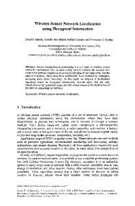
Fig. 1. (a) An N = 50 node network and the respective triangulation sets. (b) DLRE (with a decreasing weight sequence α(t) = 4/(t + 1)) results on two randomly chosen sensors from (a) showing the effect of communication noise and link failures with normalized error plot in (c). (d) DLRE (with a decreasing weight sequence, α(t) = 1/t0.55 ) results on two randomly chosen sensors from (a) showing the effect imprecise distance measurements with normalized error plot in (e).

studied in [11], converges to the exact sensor locations, even if the resulting barycentric coordinates have biased noise. V. S IMULATIONS We consider an N = 50 node network in m = 2dimensional Euclidean space (plane) with K = m+1 = 3 anchors as shown in Fig. 1(a). We assume that all of the communication links are active 90% of the time, i.e., qlj = 0.9, ∀ l s.t. j ∈ Θl , as discussed in (C2), and include an additive communication noise that is Gaussian i.i.d. with zero-mean and standard deviation 0.14 for each link. In this scenario, we employ a decreasing 4 . The results are presented weight sequence, α(t) = t+1 in Fig. 1(b) where we show the coordinate estimate for two randomly chosen sensors. We then study the effect of noisy distance measurements where the noise on each barycentric coordinate is taken to be normal with zero-mean and variance 0.1. We use a decreasing weight sequence, α(t) = 1/t0.55 , and the estimated coordinates for two arbitrarily chosen sensors is shown in Fig. 1(c) and log of the normalized mean (over the sensors) sum of the squared errors is shown in Fig. 1(d). In all of the above experiments, we can clearly see that

In this paper, we review our work on distributed sensor localization. We explicitly state our assumptions and the conditions under which the distributed algorithm converges to the exact sensor locations. We consider broad random phenomena, in particular, we consider communication link failures, communication noise and imperfect distance measurements translated to noise on the barycentric coordinates. We provide a modification to the localization algorithm using stochastic approximation and show that this modified algorithm converges a.s. under appropriate conditions. Finally, we outline the enhancements and certain modifications that can be considered to implement distributed sensor localization in more general and practical settings. R EFERENCES [1] U. A. Khan, S. Kar, and J. M. F. Moura, “Distributed sensor localization in random environments using minimal number of anchor nodes,” IEEE Transactions on Signal Processing, vol. 57, pp. 2000–2016, May 2009. [2] G. Springer, Introduction to Riemann Surfaces, AddisonWesley, Reading, MA, 1957. [3] C. Savarese, J. M. Rabaey, and J. Beutel, “Locationing in distributed ad-hoc wireless sensor networks,” in IEEE ICASSP, Salt Lake City, UA, May 2001, pp. 2037–2040. [4] M. Bawa, H. Garcia-Molina, A. Gionis, and R. Motwani, “Estimating aggregates on a peer-to-peer network,” Tech. Rep., Stanford University, 2003. [5] N. Patwari and A. O. Hero III, “Manifold learning algorithms for localization in wireless sensor networks,” in IEEE ICASSP, Montreal, Canada, Mar. 2004, pp. 857–860. [6] M. Coates, “Distributed particle filters for sensor networks,” in IEEE Information Processing in Sensor Networks, Berkeley, CA, Apr. 2004, pp. 99–107. [7] A. T. Ihler, J. W. Fisher III, R. L. Moses, and A. S. Willsky, “Nonparametric belief propagation for self-calibration in sensor networks,” in IEEE ICASSP, Montreal, Canada, May 2004. [8] M. J. Sippl and H. A. Scheraga, “Cayley–Menger coordinates,” Proceedings of the National Academy of Sciences of U.S.A., vol. 83, no. 8, pp. 2283–2287, Apr. 1986. [9] Usman A. Khan, Soummya Kar, and José M. F. Moura, “Distributed sensor localization in Euclidean spaces: Dynamic environments,” in 46th Allerton Conference On Communication, Control, and Computing, Monticello, IL, Sep. 2008. [10] Usman A. Khan, Soummya Kar, and José M. F. Moura, “Distributed localization in networks of mobile agents,” in 47th Allerton Conference On Communication, Control, and Computing, Monticello, IL, Sep. 2009, submitted. [11] Usman A. Khan, Soummya Kar, and José M. F. Moura, “Sensor localization with noisy distance measurements,” submitted to IEEE Transactions on Signal Processing, May 2009.