Distribution Map - Software Composition Group

Distribution Map In Proceedings of International Conference on Software Maintenance (ICSM 2006)

St´ephane Ducasse Language and Software Evolution Group Universit´e de Savoie, France

Tudor Gˆırba Adrian Kuhn Software Composition Group University of Berne, Switzerland

Keywords: software clustering, software metrics, visualization

system to a comparison partition1 . Typically the reference partition is the intrinsic structure of the system (e.g., the package structure of classes), and the comparison partition is given by a grouping or property (e.g., classes grouped by their authors). For example, suppose we know which developer owns which file in the system [7], we would like to answer several questions: What are the zones of interest of the developers? Is the work of a developer focused on only one part of the system, or is it scattered throughout the system? Is a package implemented by one or several developers? As another example, suppose we cluster the system based on its domain concepts [10], the questions that we would like to answer are: How are the specific concepts distributed over the package structure of the system? Are there concepts localized in one layer? Are there concepts that are spread over the entire system? Are there packages that implement one concept only? Are there packages that implement multiple concepts? In this paper, we are particularly interested in two generic questions:

1

Spread: how much does a property spread across the reference partition: is it local or global?

Abstract Understanding large software systems is a challenging task, and to support it many approaches have been developed. Often, the result of these approaches categorize existing entities into new groups or associates them with mutually exclusive properties. In this paper we present the Distribution Map as a generic technique to visualize and analyze this type of result. Our technique is based on the notion of focus, which shows whether a property is wellencapsulated or cross-cutting, and the notion of spread, which shows whether the property is present in several parts of the system. We present a basic visualization and complement it with measurements that quantify focus and spread. To validate our technique we show evidence of applying it on the result sets of different analysis approaches. As a conclusion we propose that the Distribution Map technique should belong to any reverse engineering toolkit.

Introduction

Focus: how close does a property match the reference partition: is it well-encapsulated or cross-cutting?

Understanding large and complex software is a challenging task. To address this issue, various approaches have been proposed such as software visualization [21, 11], metrics [17], or clustering [2, 13]. Often, the result of these analyses categorizes existing entities into new groups or clusters, or associates them with mutually exclusive properties. Understanding these results can be tedious as we have to understand how they are distributed over the system. Indeed, while these analyses are powerful to identify or characterize aspects of a large application, they often lack the support to understand the results they produce. In this paper we offer a generic technique to reason about the result of software analyses. Understanding how a given phenomenon is distributed across a large software system is a key information for the overall comprehension of the system. We focus on relating the reference partition of a

We introduce two measurements, as an automated means to analyze spread and focus, and we complement the measurements with a visualization that captures spread and focus of clusters or properties visually. We exemplify our technique on two different types of results: on clusters and on mutually exclusive properties. The case studies exercise different parts of the technique: first we offer an in-depth view on two case studies showing how to interpret the measurements and the visualization, and afterwards we show the scalability of the visualization on one large case study. 1 In

mathematics, a partition of a set is a division into non-overlapping parts that cover all its elements. In the context of this paper, part denotes a part of the reference partition, while cluster or property denotes a part of the comparison partition.

1

Paper structure. In Section 2 we present the technique by concentrating on its visual aspect and we define a set of metrics that complement it. In Section 3.1 we illustrate our technique on the analysis of domain concepts in Java packages, and in Section 3.2 we illustrate it on code ownership. In Section 4 we discuss the pros and cons as well as some variation points of our technique. We present the state of the art in Section 5, and we conclude in Section 6.

2

part 1

part 3

part 4

part 5

Analyzing the Distribution of Properties

Our technique has two facets. On the one hand we propose a basic visualization, the Distribution Map, and on the other hand we define a set of measurements that represent the spread and focus of properties over a partition.

2.1

part 2

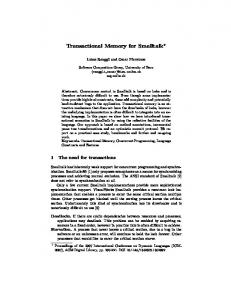
Figure 1. A Distribution Map showing five packages and four properties: Red, Blue Green and Yellow.

The Distribution Map

Given the software system S as a set of software artifacts and two partitions P and Q of that set, we introduce the Distribution Map as a means to visualize Q compared to P . The visualization is composed of large rectangles containing small squares in different colors (similar to the Shrimp views [21]). There is a small square for each element of S, the partition P is used to group the squares into large rectangles and the partition Q is used to color the squares.

with respect to their distribution over the parts. In our example from Figure 1, about the properties we say that Blue is well-encapsulated, that Yellow is cross-cutting and that Green is like an octopus because it has a body and tentacles spread over the system. We can also say that part 1 and part 4 are self-contained.

2.2

Reference partition: the partition P corresponds to a well understood partition. Typically the reference partition represents the intrinsic structure of the software system (e.g., the package structure). However, we could also use the result of a clustering.

Measuring Spread and Focus

In addition to the visualization we introduce two measurements to quantifying both the spread and the focus of a property q in relation to a partition P . The set of elements in part p ∈ P that have property q is the intersection between property q and part p. Its relative size can either be given in terms of a percentage of p or in terms of a percentage of q, thus we define the relative size of q ∩ p in relation to p as:

Comparison partition: the partition Q is the result of an analysis. Mostly, this partition is either a set of clusters, or some mutually exclusive properties associated with the elements of S.

touch(q, p) := In the context of this paper, to distinguish the comparison partition from the reference partition, we call the parts of the comparison partition properties (the terms cluster and property are used synonymously in this paper). Thus, we say that each software artifact si belongs to a part pn of P and is attributed with a property qm out of Q. Figure 1 illustrates an example Distribution Map with five parts containing 6, 2, 5, 10 and 14 elements respectively and with four properties: Red, Blue, Green and Yellow. On the visualization, for each part pn there is a large rectangle and within that rectangle, for each element si ∈ pn there is a small square whose color refers to the property qm attributed to that element. From the visualization we can characterize both the parts with respect to the contained properties, and the properties

|q ∩ p| |p|

The name relative size is generic, when applying the Distribution Map on a specific result set its problem domain usually provides a more accurate vocabulary. For example, in the case of authorship we would say “percentage of package B touched by author A”. Spread. Given the total set S, a subset of elements q ⊂ S and a partition P such that ∪P = S, we define the spread of q over P as the number of touched parts: X  1, touch(q, pi ) > 0 spread(q, P ) := 0, touch(q, pi ) = 0 pi ∈P

2

Focus. Given again the total set S, a subset of elements q ⊂ S and a partition P such that ∪P = S, we define the focus of q on the touched parts of P as: X focus(q, P ) := touch(q, pi ) ∗ touch(pi , q)

tion Map on software clustering. The semantic partition of a system, as obtained by semantic clustering, does generally not correspond one-to-one to its structural modularization. In most systems we find both concepts that correspond to the structure and concepts that cross-cut it [10].

pi ∈P

The focus is a number between 0 and 1 and measures the distance between the subset q and the partition P : the larger the number, the more the parts touched by q are touched entirely by q. This means that well-encapsulated properties have a high focus value, and cross-cutting properties have a low focus value. Note that the notion of focus differs from the notion of cohesion: focus characterizes a property, while cohesion characterizes the internals of a part.

3.1.1

JEdit is a text editor written in Java, the source has a total of 394 classes in 31 packages and uses a vocabulary of 1603 distinct terms, applying semantic clustering results in nine domain concepts [10]. Figure 2 illustrates how the retrieved domain concepts are distributed over the package structure: the parts are the packages, the elements are the classes and the colors refer to their concepts. The table below lists for each concept its size, its spread, its focus and a description of its concept.

Example. The table below lists the size, the spread and the focus of each property from the Figure 1: color red blue green yellow

size 15 11 9 3

spread 2 1 4 3

focus .80 1.0 .75 .25

color red blue cyan green pink dark-green yellow magenta orange

description main property well-encapsulated octopus cross-cutting

The table reinforces what we detected in Figure 1. For example, we characterize Blue as being well-encapsulated because it has a high focus, and we characterize Yellow as being cross-cutting because it has a low focus and high spread.

3

size 116 80 68 63 26 12 10 10 9

spread 25 4 8 13 7 3 4 3 1

focus .605 .883 .712 .475 .335 .456 .105 .484 .900

concept (main domain concept) BeanShell scripting regular expressions user interface text buffers TAR and ZIP archives dockable windows XML reader bytecode assembler

Looking at the Numbers. The three most wellencapsulated concepts, that is the clusters with the highest focus (Orange, Blue and Cyan), implement clearly separated concepts such as scripting and regular expressions. The concepts with the lowest focus cross-cut the system: Yellow implements dockable windows, a custom GUI-feature, and Pink is about handling text buffers. These two concepts are good candidates for a closer inspection, since we might want to refactor them into packages of their own.

Application of the Distribution Map

In this section we apply the Distribution Map on the results of two analyses: (1) the distribution of domain concepts over Java packages, and (2) the distribution of code ownership over folders. The intent of this section is to evaluate the Distribution Map as an exploration tool when applied on the result of automated analysis. The discussion of the actual analyses is out if the scope of this paper. For an in-depth understanding of the details we refer the reader to papers already published by the authors [7, 10]. The case studies exercise different parts of the technique: in the case of semantic analysis we offer an in-depth view on two case studies showing how to interpret the measurements and the visualization, while in the case of code ownership analysis we show the scalability of the visualization on one large case study.

3.1

Semantic Clustering of JEdit

Looking at the Distribution Map. In Figure 2 the distribution of Red, the largest cluster and thus the main domain concept of the application, shows which parts of the system belong to the core and which do not. Based on the ordering of the packages, we can conclude that the two UI concepts, Green and Yellow, are more closely related to the core than for example concept Cyan, which implements regular expressions. 3.1.2

Application: Distribution of Linguistic Concepts in Software Systems

Semantic Clustering of Ant

Ant is a popular development tool for Java. Its source has a total of 665 classes in 66 packages and uses a vocabulary of 1787 distinct terms. Applying semantic clustering resulted in nine domain concepts [10]. Figure 3 illustrates how the

As a first showcase we employ Semantic Clustering on two case studies to illustrate the application of the Distribu3

Figure 2. Distribution Map of linguistic concepts over the packages of JEdit 31 parts, 394 elements and 9 properties).

retrieved domain concepts are distributed over the package structure of the system. color red blue cyan green pink orange yellow magenta black

size 390 103 56 48 23 21 15 7 3

spread 47 22 7 10 9 6 4 2 3

focus .808 .555 .803 .421 .557 .210 .904 1.0 .087

plug-ins such as the Pink parts, which implement network protocols, or the Cyan and Magenta parts, which implement plug-ins for different version control systems.

concept (main domain concept) string processing version control clients unit-test support network protocols XML handling image and graphics another versioning client FTP and filesystem

3.2

Application: The Distribution of File Ownership

As second showcase we apply Distribution Map on a different domain (i.e., code ownership analysis) and we focus on the scalability of the visualization by studying a large case study (JBoss). As a further difference to the previous showcase, the comparison partition of this case study is not the result of a clustering algorithm, but is the result of attaching a property to each artifact. In this case, the artifacts are the files, and the properties are the owner of the file. To obtain the owner of a file, we use the heuristic that a file is owned by the developer that wrote the most lines of code in that file [7]. JBoss2 is an open source Java application server. The CVS repository goes back five years beginning in April 2000 and contains about 2700 files summing up over 25000 revisions. The system is written by 133 authors, and 14 of them have implemented over 80% of the lines. Thus we select those 14 to be shown on the visualization as colored properties, and leave the remaining properties grayed out. Figure 4 shows how the files owned by these authors are distributed over the file-folder structure: the parts are the folders that ever existed in the system, the elements are the file that ever existed in the system and the colors refer to the owners.

The table above lists for each cluster its size, its spread, its focus and a description of its concept. Looking at the Numbers. The four concepts with the lowest focus value, Blue, Green, Orange and Pink, crosscut the package structure and implement main features of a development tool: string processing, unit-testing and XML handling. Other features, such as access to version control systems and network protocols, are well-encapsulated in concepts with a high focus number. Looking at the Distribution Map. The order of the packages is not arbitrary or by name, but reflects the distribution of the concepts. The packages are ordered using dendrogram seriation (see Section 4.2). On the first three rows there are packages that implement the core functionality of Ant, the largest concept which is Red, dominates this part of the figure. Then, on row four we find the octopus concepts Blue and Green that are used by the core packages in the third row. And, on the last row there are well-encapsulated

2 JBoss

4

CVS-repository, Nov. 2005, http://www.jboss.org.

Figure 3. Distribution Map of linguistic concepts over the packages of Ant (66 parts, 665 elements and 9 properties).

color red cyan blue magenta orange purple green

size 279 194 187 145 130 120 115

spread 61 23 19 21 11 15 35

focus .416 .796 .857 .546 .934 .437 .282

color pink brown royal yellow d’green olive navy

size 102 99 79 72 69 69 60

spread 30 28 21 24 12 21 14

focus .349 .325 .692 .193 .312 .738 .829

are all-rounders as well as specialists among the main developers of the system. The two authors with the lowest focus, Green and Yellow, cross-cut the system touching about 30 parts, while the author with the next lowest focus, which is Dark green, touches only 12 folders. On the other end of the spectrum there are Orange, Blue and Navy as most focused authors, each of them owns a dozen parts just by themselves, and author Red, that owns the most files and touches a third of the system but with a moderate focus.

The table above lists for each author, its color on the figure, the number of files he owns, and both the spread and the focus of its ownership.

Variation point. In Figure 5 we show a variation of Figure 4 where we use the same layout, but we show the number of commits on the files. We employed the heat scale: Red denotes more than 50 commits, Yellow more than 20 commits, and Light blue less than 20 commits. The figure is zoomed out to the size of a thumbnail and contains 2000 elements: yet it is still readable.

Looking at the Distribution Map. There are over 2000 elements and 200 parts, yet the visualization still scales. Only the top 14 authors are colored, the remaining are left out in light gray. Folders that have been written by one author are clearly distinguishable from folders written by teams. We can identify the focus authors that worked on separate parts of the system, as well as the cross-cutters that spread over the system.

4 Looking at the Numbers. Even if the comparison partition of this case study results from an approach that fundamentally differs from clustering, the two metrics focus and spread make sense as well. The focus metric for example covers the whole ranges from 0.1 to 0.9, revealing that there

Discussion

In this section we discuss the applicability of the Distribution Map, we abstract some recurring patterns we observed from our experiments, and we discuss the most important design decisions for the visualization. 5

Figure 4. Distribution Map of the file ownership of JBoss during five years (204 parts, 2107 elements and 15 properties).

6

Characterizing the parts. following patterns:

For the parts we identified the

• Single property. It denotes a part in which all elements have the same property. Other parts may have elements with the same property. We identified this case in all the three case studies. For example, in Figure 4 almost all the bottom right folders are written entirely by Orange. • Unique property. It denotes a part in which its elements have a property that no other part has in the system. In Figure 2, the third package of the third row has five classes with properties unique in the system. • Dominant property. It denotes a part in which nearly all the elements have a certain property. In Figure 3, Red is characterized as having a dominant property. • Property Assembler. It denotes a part that contains elements showing most of the properties present in the system. In Figure 2, the fifth package of the fourth row has the most properties of the system, and in Figure 4 the fourth folder from the right on the third row (named ejb) was touched by most of the developers. Figure 5. Distribution Map of the number of commits in JBoss (204 parts, 2107 elements and 3 properties).

Characterizing the properties. identified the following patterns:

• Well-encapsulated. If a property corresponds to the structure, we call this a well-encapsulated concept. Such a concept is spread over one or multiple modules, and includes almost all artifacts within those modules. In Figure 3 Yellow is well encapsulated.

In the previous sections we exemplified our technique on two common types of analysis results: clustering and properties. However, our technique is more generic and it can be applied to any two partitions of the system: one partition as a reference, and the other for comparison. The simplest case for a comparison partition is a boolean partition splitting the elements into two distinct sets based on the conformity to a certain property. Furthermore, having two partitions, the Distribution Map can be applied in both directions by inverting the reference with the comparison partition. For example, in the case of software clustering we can either choose the structure as reference and compare it to the clustering, or the other way round, take the clustering as reference and relate it to the structure as comparison partition.

4.1

For the properties we

• Cross-Cutting. If a property is spread over several parts but only touches them slightly, we call crosscutting. In Figure 4 the Yellow author is changing bits and pieces everywhere, and in Figure 2 the Pink concept cross-cuts several packages. • Black Sheep. If there is a property that cross-cuts the system, but it touches very few elements, we call it a black sheep. In Figure 3 Black is such a black sheep. • Octopus. If a property is well encapsulated in a few parts, but also spreads across other parts, as a crosscutter does, we call this an octopus. In Figure 3 Green covers the JUnit plugin implementation package and also spreads over several other packages.

Recurring Patterns

4.2 Based on our experiments, we develop a vocabulary to describe the recurring patterns we encountered. The vocabulary covers both the characterization of the parts as compared with the properties they contain and the characterization of the properties with respect to the parts they touch.

Visual Design Decisions

The visualization we propose looks simple. The simplicity of the visualization is an important characteristic because we want it to be useful for software engineers without much training in visualization [12]. This visualization 7

On the choice of colors. The choice of colors affects the readability of the Distribution Map as well. We need to pay attention to the characteristic of human vision to make sure that the visualization is easy to read and to avoid wrong conclusions. First, scattered squares are easier to spot if they are shown in distinct colors than if they are shown in colors similar to the well-encapsulated colors. Therefore light colors are a good choice for cross-cutting concerns and dark colors a good choice for well encapsulated concepts. Second, a human reader will draw conclusions concerning the similarity between concepts based on the similarity of the colors that denote these concepts. For example, green and dark green suggest that two concepts are related, while green and red suggest that the same two concepts are unrelated. Therefore, it is recommended to take domain specific similarities into account when choosing the colors. For example, in the case of software clustering, more similar clusters have more similar colors and vice versa.

is simple to draw and then to reproduce, simple to interpret and can convey a reasonable amount of information in a limited amount of space. On the arrangement of the part-boxes. The order of the parts is crucial, since the layout determines whether distribution patterns are easily recognizable or not. The location of the parts given by the structure is not necessarily the best choice: using an arbitrary order, as for example by name or directory structure, most patterns get lost as they are scattered too sparsely over the structure. Therefore, we prefer an ordering where parts with similar properties are placed near each other. To achieve this ordering we use dendrogram seriation, a clustering technique that orders items such that similar items are placed near each other according to a similarity metric [18]. In our case, we define the similarity between two parts as the cosine between their feature vectors: two parts are more similar if the ratios between their respective properties match. The feature vector v of a part p lists for each property qi the number of touched elements in that part. In Figure 1, part 3 has three red, no blue, one green and one yellow element, thus its feature vector is v = (3, 0, 1, 1). This vector is more similar to part 2 (v = (0, 0, 1, 1)) and with part 4 (v = (12, 0, 1, 1)) which are therefore placed next to it, and it is not similar to part 5 ( v = (0, 10, 0, 0)) which is therefore placed in the opposite corner. This layout strategy enables a spatial interpretation of the visualization: quantifications such as far apart or near each other become a meaningful interpretation, relational information is expressed in spatial terms. This makes the Distribution Map a real map. The location of both the parts and the properties reflect their relation among and between each other. For example, even if two related properties never appear together in the same part, the layout algorithm places them nonetheless near each other on the map, provided that both co-occur somewhere with other properties.

On the limitation of colors. The study of human perception shows that there are only eight colors which are recalled by humans with more than 75% probability. This means that we can not discriminate more than a dozen different colors at once [25], which puts an upper limit on the number of properties being displayed on the Distribution Map. Sometimes it is possible to work around this limitation using the Pareto principle, which is the well known rule-of-thumb that for many phenomena, 80% of the consequences stem from 20% of the causes. See for example the case study in Section 3.2, where 80% of the systems code is written by only 14 out of 133 authors.

5

Related Work

Graphical representations of software have long been accepted as comprehension aids. Lanza and Ducasse present polymetrics views, simple visualizations enriched by metrics [4, 12]. Polymetric views are powerful since the simple visualizations are scalable and semantics is added via the combination of metrics. The difference with the current work is that we focus on analyzing nominal properties, while polymetric views focus on analyzing metrics. SV3D, developed by Marcus et al, presents lines of code as dots and each dot can be associated with different information such as the nesting level or the control flow [14]. For quantitative information, such as the occurrence of a phenomena, 3D is used. Their approach is close to ours. however in their case the parts and the elements are ordered by file name and source line, while in our case we put them in a more comprehensive order such that pattern become more visible. Microprints are a dot-based representation of method bodies [19]. Microprints are similar to Seesoft [6] visual-

On the shape of part-boxes. We experimented with several shapes, but in the end we designed an algorithm to produce rectangles with dimensions close to the ratio of the golden mean [23]. On the arrangement of the element-boxes. Inside the packages we group the elements by properties, and use in each package the same order. That is, for example on Figure 5, the red elements come first, then the yellow ones, and then the blue ones. This layout has two advantages: it is easy to tell the number of elements with the same property, and as the properties are always placed in the same order, one can compare different parts easier. 8

6

ization and follow the source code to conserve familiarity. Similarly Control Structure Diagrams [9] are also based on the layout of the code since they are intended to support the programmers to understand the flow and structure of methods. These approaches are different from ours since they focuses bringing more information at the code structure level.

Conclusion

Analyzing a system means decomposing it into significant parts. Different analyses will decompose a system in different ways. Examples of such analyses are clustering or grouping, where the results of such methods are groups of elements from the system that share common properties. In this paper, we address the problem of reasoning about these results.

Ducasse, Lanza and Ponisio butterfly’s visualization goal is to characterize packages in a fine grained manner by providing a compact view based on seven different measurements [5]. Sharble and Cohen introduce a compass-type plot for eight metrics [20]. Chuah and Eick visualize project information through glyphs [3]. They use glyphs for viewing project management data (i.e., evolution aspects, programming languages used, and errors found in a software component). The work presented in this paper is different since we focused on the concept of spread and containment i.e., how a given phenomenon distributes over a system and its constituents.

We develop the concept of Distribution Map and propose a visualization and two measurements to analyze the distribution of properties over the reference partition. Based on our practice with the Distribution Map technique we provide a vocabulary to characterize reoccurring pattern of both partition and properties. This vocabulary, as well as the development of the technique in general, is distilled from practical experience with the results of automated software analyses.

Using measurements is another widely spread approach to assess unknown systems. Hautus introduced Pasta, a tool to analyze the structure of Java programs and a metric to determine the quality of the package architecture [8]. Allen et al, defined information theory-based – as opposed to counting – coupling and cohesion metrics for modules [1] that are represented as graphs. They define module and intramodule in terms of the subgraph’s information and cohesion in terms of intra-module coupling.

We paid special attention to presenting the decisions we took when designing the visualization. Even if it looks simple, there are a couple of important attributes of it, in particular the layout of the part-boxes and the choice of colors. Due to its layout the Distribution Map is indeed a map showing relational information in a spatial space: distance quantifications such as far away or near each other do have a meaningful interpretation. Related parts and properties are placed near each other, while unrelated parts or properties are placed far apart.

Marinescu defined detection strategies as metric-based expressions to detect design flaws [15]. Our technique can be used to display the design flaws over the system.

To validate our technique, we apply it on the results of two distinct analyses (semantic analysis and ownership analysis) to exercise different facets of it: readability and scalability of the visualization, and correlation between the visualization and the proposed measurements. We show that the Distribution Map is a generic tool and applicable on a broad range of software analyses.

Another related area is the one of clustering. Tzerpos and Hold compare the results of software clustering using a distance measurement [24]. They present the MoJo-distance, a distance metric that compares entire partitions and tells only how close one partition is to another. Their approach is much more coarse than ours, as we zoom into the details and measure how the specific parts of the comparison partition are spread over the reference partition. Tonella introduces a distance metric as well, which focuses on the cost of restructuring the system from [22]. Both approaches define the distance as the minimal number of elementary operation required to transform the first partition into the second partition.

The technique provides a quick look at the distribution of properties within a system, and it uncovers complex information in an intuitive way. The Distribution Map is meant to fill the gap between the raw results obtained by automated algorithms and the following analysis carried out by a human expert. The Distribution Map is an eclectic approach that combines an intuitive visualization and straightforward metrics into a generic and easy-to-use tool. It is this combination that makes the Distribution Map a good starting point to reason about the results of automated algorithms, and should as such belong to any reverse engineering toolkit.

Similar to our layout strategy, Merkl used self organizing maps (SOM) to arrange software project on a 2D plane based on some distance metric [16]. Self organizing maps are an artificial intelligence technique based on neutral networks: they are good at producing 2D layouts of highdimensional data. Our technique uses a similar layout strategy but with another focus, we do not aim at the similarity between parts but at revealing pattern in the distribution of properties.

In the future, we plan to continue to apply the Distribution Map in the context of different analyses. Furthermore, we plan to explore the effect of other layouts strategies on the spatial space of the visualization. 9

Acknowledgments. We gratefully acknowledge the financial support of the Swiss National Science Foundation for the project Recast: Evolution of Object-Oriented Applications (SNF 2000-061655.00/1) and french ANR for the Cook: rearchitecturing object-oriented applications.

[13] J. I. Maletic and A. Marcus. Supporting program comprehension using semantic and structural information. In Proceedings of the 23rd International Conference on Software Engineering (ICSE 2001), pages 103–112, May 2001. [14] M. Marchesi and G. Succi, editors. Extreme Programming and Agile Processes in Software Engineering. Springer, 2003. [15] R. Marinescu. Detection strategies: Metrics-based rules for detecting design flaws. In 20th IEEE International Conference on Software Maintenance (ICSM’04), pages 350–359, Los Alamitos CA, 2004. IEEE Computer Society Press. [16] D. Merkl. Content-based software classification by selforganization. In Proceddings of International Conference on Neural Networks (ICNN’95), volume II, pages 1086–1091, 1995. [17] T. Miceli, H. A. Sahraoui, and R. Godin. A metric based technique for design flaws detection and correction. In Proceedings IEEE Automated Software Engineering Conference (ASE), 1999. [18] S. Morris, B. Asnake, and G. Yen. Dendrogram seriation using simulated annealing. Information Visualization, 2(2):95–104, 2003. [19] R. Robbes, S. Ducasse, and M. Lanza. Microprints: A pixelbased semantically rich visualization of methods. In Proceedings of ESUG 2005 (13th International Smalltalk Conference), pages 131–157, 2005. [20] R. C. Sharble and S. S. Cohen. The object-oriented brewery: a comparison of two object-oriented development methods. SIGSOFT Softw. Eng. Notes, 18(2):60–73, 1993. [21] M.-A. D. Storey and H. A. M¨uller. Manipulating and Documenting Software Structures using SHriMP Views. In Proceedings of ICSM ’95 (International Conference on Software Maintenance), pages 275–284. IEEE Computer Society Press, 1995. [22] P. Tonella. Concept Analysis for Module Restructuring. IEEE Transactions on Software Engineering, 27(4):351– 363, Apr. 2001. [23] E. R. Tufte. The Visual Display of Quantitative Information. Graphics Press, 2nd edition, 2001. [24] V. Tzerpos and R. Holt. MoJo: A distance metric for software clusterings. In Proceedings Working Conference on Reverse Engineering (WCRE 1999), pages 187–195, Los Alamitos CA, 1999. IEEE Computer Society Press. [25] C. Ware. Information Visualization. Morgan Kaufmann, 2000.

References [1] E. Allen and T. Khoshgoftaar. Measuring coupling and cohesion of software modules: An information theory approach. In Seventh International Software Metrics Symposium, 2001. [2] N. Anquetil and T. Lethbridge. Experiments with Clustering as a Software Remodularization Method. In Proceedings of WCRE ’99 (6th Working Conference on Reverse Engineering), pages 235–255, 150 Louis Pasteur, University of Ottawa, Ottawa, Canada, 1999. [3] M. C. Chuah and S. G. Eick. Information rich glyphs for software management data. IEEE Computer Graphics and Applications, 18(4):24–29, July 1998. [4] S. Demeyer, S. Ducasse, and M. Lanza. A hybrid reverse engineering platform combining metrics and program visualization. In F. Balmas, M. Blaha, and S. Rugaber, editors, Proceedings WCRE ’99 (6th Working Conference on Reverse Engineering). IEEE, Oct. 1999. [5] S. Ducasse, M. Lanza, and L. Ponisio. Butterflies: A visual approach to characterize packages. In Proceedings of the 11th IEEE International Software Metrics Symposium (METRICS’05). IEEE Computer Society, 2005. [6] S. G. Eick, J. L. Steffen, and S. Eric E., Jr. SeeSoft—a tool for visualizing line oriented software statistics. IEEE Transactions on Software Engineering, 18(11):957–968, Nov. 1992. [7] T. Gˆırba, A. Kuhn, M. Seeberger, and S. Ducasse. How developers drive software evolution. In Proceedings of International Workshop on Principles of Software Evolution (IWPSE 2005), pages 113–122. IEEE Computer Society Press, 2005. [8] E. Hautus. Inmproving Java software through package structure analysis. In International Conference Software Engineering and Applications, 2002. [9] D. Hendrix, J. H. Cross II, and S. Maghsoodloo. The Effectiveness of Control Structure Diagrams in Source Code Comprehension Activities. IEEE Transactions on Software Engineering, 28(5):463–477, May 2002. [10] A. Kuhn, S. Ducasse, and T. Gˆırba. Enriching reverse engineering with semantic clustering. In Proceedings of Working Conference on Reverse Engineering (WCRE 2005), pages 113–122, Los Alamitos CA, Nov. 2005. IEEE Computer Society Press. [11] M. Lanza. Codecrawler — lessons learned in building a software visualization tool. In Proceedings of CSMR 2003, pages 409–418. IEEE Press, 2003. [12] M. Lanza and S. Ducasse. Polymetric views—a lightweight visual approach to reverse engineering. IEEE Transactions on Software Engineering, 29(9):782–795, Sept. 2003.

10