Dominant Sets for “Constrained” Image Segmentation - arXiv

1

Dominant Sets for “Constrained” Image Segmentation

arXiv:1707.05309v1 [cs.CV] 15 Jul 2017

Eyasu Zemene, Member, IEEE, Leulseged Tesfaye Alemu, Member, IEEE and Marcello Pelillo, Fellow, IEEE Abstract—Image segmentation has come a long way since the early days of computer vision, and still remains a challenging task. Modern variations of the classical (purely bottom-up) approach, involve, e.g., some form of user assistance (interactive segmentation) or ask for the simultaneous segmentation of two or more images (co-segmentation). At an abstract level, all these variants can be thought of as “constrained” versions of the original formulation, whereby the segmentation process is guided by some external source of information. In this paper, we propose a new approach to tackle this kind of problems in a unified way. Our work is based on some properties of a family of quadratic optimization problems related to dominant sets, a well-known graph-theoretic notion of a cluster which generalizes the concept of a maximal clique to edge-weighted graphs. In particular, we show that by properly controlling a regularization parameter which determines the structure and the scale of the underlying problem, we are in a position to extract groups of dominant-set clusters that are constrained to contain predefined elements. In particular, we shall focus on interactive segmentation and co-segmentation (in both the unsupervised and the interactive versions). The proposed algorithm can deal naturally with several type of constraints and input modality, including scribbles, sloppy contours, and bounding boxes, and is able to robustly handle noisy annotations on the part of the user. Experiments on standard benchmark datasets show the effectiveness of our approach as compared to state-of-the-art algorithms on a variety of natural images under several input conditions and constraints. Index Terms—Interactive segmentation, co-segmentation, dominant sets, quadratic optimization, game dynamics.

F

1

I NTRODUCTION

I

MAGE segmentation is arguably one of the oldest and best-studied problems in computer vision, being a fundamental step in a variety of real-world applications, and yet remains a challenging task [1] [2]. Besides the standard, purely bottom-up formulation, which involves partitioning an input image into coherent regions, in the past few years several variants have been proposed which are attracting increasing attention within the community. Most of them usually take the form of a “constrained” version of the original problem, whereby the segmentation process is guided by some external source of information. For example, user-assisted (or “interactive”) segmentation has become quite popular nowadays, especially because of its potential applications in problems such as image and video editing, medical image analysis, etc. [3], [4], [5], [6], [7], [8], [9]. Given an input image and some information provided by a user, usually in the form of a scribble or of a bounding box, the goal is to provide as output a foreground object in such a way as to best reflect the user’s intent. By exploiting high-level, semantic knowledge on the part of the user, which is typically difficult to formalize, we are therefore able to effectively solve segmentation problems which would be otherwise too complex to be tackled using fully automatic segmentation algorithms. Existing algorithms fall into two broad categories, depending on whether the user annotation is given in terms of

•

The authors are with the Dipartimento di Scienze Ambientali, Informatica e Statistica, Universita Ca’ Foscari Venezia, via Torino 155, 30172 Venezia Mestre, Italy. E-mail: {eyasu.zemene, leuelseged, pelillo}@unive.it

a scribble or of a bounding box, and supporters of the two approaches have both good reasons to prefer one modality against the other. For example, Wu et al. [5] claim that bounding boxes are the most natural and economical form in terms of the amount of user interaction, and develop a multiple instance learning algorithm that extracts an arbitrary object located inside a tight bounding box at unknown location. Yu et al. [10] also support the bounding-box approach, though their algorithm is different from others in that it does not need bounding boxes tightly enclosing the object of interest, whose production of course increases the annotation burden. They provide an algorithm, based on a Markov Random Field (MRF) energy function, that can handle input bounding box that only loosely covers the foreground object. Xian et al. [11] propose a method which avoids the limitations of existing bounding box methods region of interest (ROI) based methods, though they need much less user interaction, their performance is sensitive to initial ROI. On the other hand, several researchers, arguing that boundary-based interactive segmentation such as intelligent scissors [9] requires the user to trace the whole boundary of the object, which is usually a time-consuming and tedious process, support scribble-based segmentation. Bai et al. [12], for example, propose a model based on ratio energy function which can be optimized using an iterated graph cut algorithm, which tolerates errors in the user input. In general, the input modality in an interactive segmentation algorithm affects both its accuracy and its ease of use. Existing methods work typically on a single modality and they focus on how to use that input most effectively. However, as noted recently by Jain and Grauman [13], sticking to

2

one annotation form leads to a suboptimal tradeoff between human and machine effort, and they tried to estimate how much user input is required to sufficiently segment a novel input. Another example of a “constrained” segmentation problem is co-segmentation. Given a set of images, the goal here is to jointly segment same or similar foreground objects. The problem was first introduced by Rother et al. [14] who used histogram matching to simultaneously segment the foreground object out from a given pair of images. Recently, several techniques have been proposed which try to cosegment groups containing more than two images, even in the presence of similar backgrounds. Joulin et al. [15], for example, proposed a discriminative clustering framework, combining normalized cut and kernel methods and the framework has recently been extended in an attempt to handle multiple classes and a significantly larger number of images [16]. The co-segmentation problem has also been addressed using user interaction [17], [18]. Here, a user adds guidance, usually in the form of scribbles, on foreground objects of some of the input images. Batra et al. [17] proposed an extension of the (single-image) interactive segmentation algorithm of Boykov and Jolly [8]. They also proposed an algorithm that enables users to quickly guide the output of the co-segmentation algorithm towards the desired output via scribbles. Given scribbles, both on the background and the foreground, on some of the images, they cast the labeling problem as energy minimization defined over graphs constructed over each image in a group. Dong et al. [18] proposed a method using global and local energy optimization. Given background and foreground scribbles, they built a foreground and a background Gaussian mixture model (GMM) which are used as global guide information from users. By considering the local neighborhood consistency, they built the local energy as the local smooth term which is automatically learned using spline regression. The minimization problem of the energy function is then converted into constrained quadratic programming (QP) problem, where an iterative optimization strategy is designed for the computational efficiency. In this paper (which is an extended version of [19]), we propose a unified approach to address this kind of problems which can deal naturally with various type of input modality, or constraints, and is able to robustly handle noisy annotations on the part of the external source. In particular, we shall focus on interactive segmentation and cosegmentation (in both the unsupervised and the interactive versions). Our approach is based on some properties of a parameterized family of quadratic optimization problems related to dominant-set clusters, a well-known generalization of the notion of maximal cliques to edge-weighted graph which have proven to be extremely effective in a variety of computer vision problems, including (automatic) image and video segmentation [20], [21] (see [22] for a recent review). In particular, we show that by properly controlling a regularization parameter which determines the structure and the scale of the underlying problem, we are in a position to extract groups of dominant-set clusters which are constrained to contain user-selected elements. We provide bounds that allow us to control this process, which

are based on the spectral properties of certain submatrices of the original affinity matrix. The resulting algorithm has a number of interesting features which distinguishes it from existing approaches. Specifically: 1) it is able to deal in a flexible manner with both scribble-based and boundary-based input modalities (such as sloppy contours and bounding boxes); 2) in the case of noiseless scribble inputs, it asks the user to provide only foreground pixels; 3) it turns out to be robust in the presence of input noise, allowing the user to draw, e.g., imperfect scribbles (including background pixels) or loose bounding boxes. Experimental results on standard benchmark datasets demonstrate the effectiveness of our approach as compared to state-of-the-art algorithms on a wide variety of natural images under several input conditions. Figure 1 shows some examples of how our system works in both interactive segmentation, in the presence of different input annotations, and co-segmentation settings.

2

D OMINANT SETS AND QUADRATIC OPTIMIZATION

In the dominant set framework, the data to be clustered are represented as an undirected edge-weighted graph with no self-loops G = (V, E, w), where V = {1, ..., n} is the ∗ vertex set, E ⊆ V × V is the edge set, and w : E → R+ is the (positive) weight function. Vertices in G correspond to data points, edges represent neighborhood relationships, and edge-weights reflect similarity between pairs of linked vertices. As customary, we represent the graph G with the corresponding weighted adjacency (or similarity) matrix, which is the n × n nonnegative, symmetric matrix A = (aij ) defined as aij = w(i, j), if (i, j) ∈ E , and aij = 0 otherwise. Since in G there are no self-loops, note that all entries on the main diagonal of A are zero. For a non-empty subset S ⊆ V , i ∈ S , and j ∈ / S , define X 1 φS (i, j) = aij − aik . (1) |S| k∈S This quantity measures the (relative) similarity between nodes j and i, with respect to the average similarity between node i and its neighbors in S . Note that φS (i, j) can be either positive or negative. Next, to each vertex i ∈ S we assign a weight defined (recursively) as follows: ( 1, if |S| = 1, wS (i) = P φ (j, i)w (j), otherwise . S\{i} S\{i} j∈S\{i} (2) Intuitively, wS (i) gives us a measure of the overall similarity between vertex i and the vertices of S \ {i} with respect to the overall similarity among the vertices in S\{i}. Therefore, a positive wS (i) indicates that adding i into its neighbors in S will increase the internal coherence of the set, whereas in the presence of a negative value we expect the overall coherence to be decreased. Finally, the total weight of S can be simply defined as X W (S) = wS (i) . (3) i∈S

A non-empty subset of vertices S ⊆ V such that W (T ) > 0 for any non-empty T ⊆ S , is said to be a dominant set if:

3

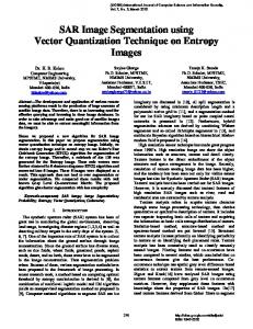
Fig. 1: Left: An example of our interactive image segmentation method and its outputs, with different user annotation. Respectively from top to bottom, tight bounding box (Tight BB), loose bounding box (Loose BB), a scribble made (only) on the foreground object (Scribble on FG) and scribbles with errors. Right: Blue and Red dash-line boxes, show an example of our unsupervised and interactive co-segmentation methods, respectively. 1) 2)

3

wS (i) > 0, for all i ∈ S , wS∪{i} (i) < 0, for all i ∈ / S.

It is evident from the definition that a dominant set satisfies the two basic properties of a cluster: internal coherence and external incoherence. Condition 1 indicates that a dominant set is internally coherent, while condition 2 implies that this coherence will be destroyed by the addition of any vertex from outside. In other words, a dominant set is a maximally coherent data set. Now, consider the following linearly-constrained quadratic optimization problem: maximize subject to

f (x) = x0 Ax x∈∆

(4)

where a prime denotes transposition and ( ) n X ∆ = x ∈ Rn : xi = 1, and xi ≥ 0 for all i = 1 . . . n i=1

is the standard simplex of Rn . In [20], [21] a connection is established between dominant sets and the local solutions of (4). In particular, it is shown that if S is a dominant set then its “weighted characteristics vector,” which is the vector of ∆ defined as, ( w (i) S , if i ∈ S, xi = W (s) 0, otherwise is a strict local solution of (4). Conversely, under mild conditions, it turns out that if x is a (strict) local solution of program (4) then its “support”

σ(x) = {i ∈ V : xi > 0} is a dominant set. By virtue of this result, we can find a dominant set by first localizing a solution of program (4) with an appropriate continuous optimization technique, and then picking up the support set of the solution found. In this sense, we indirectly perform combinatorial optimization via continuous optimization. A generalization of these ideas to hypergraphs has recently been developed in [23].

C ONSTRAINED DOMINANT SETS

Let G = (V, E, w) be an edge-weighted graph with n vertices and let A denote as usual its (weighted) adjacency matrix. Given a subset of vertices S ⊆ V and a parameter α > 0, define the following parameterized family of quadratic programs: maximize subject to

fSα (x) = x0 (A − αIˆS )x x∈∆

(5)

where IˆS is the n × n diagonal matrix whose diagonal elements are set to 1 in correspondence to the vertices contained in V \ S and to zero otherwise, and the 0’s represent null square matrices of appropriate dimensions. In other words, assuming for simplicity that S contains, say, the first k vertices of V , we have:   0 0 ˆ IS = 0 In−k where In−k denotes the (n−k)×(n−k) principal submatrix of the n × n identity matrix I indexed by the elements of V \ S . Accordingly, the function fSα can also be written as follows: fSα (x) = x0 Ax − αx0S xS

xS being the (n − k)-dimensional vector obtained from x by dropping all the components in S . Basically, the function fSα is obtained from f by inserting in the affinity matrix A the value of the parameter α in the main diagonal positions corresponding to the elements of V \ S . Notice that this differs markedly, and indeed generalizes, the formulation proposed in [24] for obtaining a hierarchical clustering in that here, only a subset of elements in the main diagonal is allowed to take the α parameter, the other ones being set to zero. We note in fact that the original (nonregularized) dominant-set formulation (4) [21] as well as its regularized counterpart described in [24] can be considered as degenerate version of ours, corresponding to the cases S = V and S = ∅, respectively. It is precisely this increased flexibility which allows us to use this idea for finding groups of “constrained” dominant-set clusters.

4

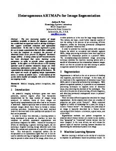
Fig. 2: An example graph (left), corresponding affinity matrix (middle), and scaled affinity matrix built considering vertex 5 as a user constraint (right). Notation Ci refers to the ith maximal clique.

We now derive the Karush-Kuhn-Tucker (KKT) conditions for program (5), namely the first-order necessary conditions for local optimality (see, e.g., [25]). For a point x ∈ ∆ to be a KKT-point there should exist n nonnegative real constants µ1 , . . . , µn and an additional real number λ such that [(A − αIˆS )x]i − λ + µi = 0 for all i = 1 . . . n, and n X

Hence, (Ax)i > x0 Ax−αx0S xS for i ∈ / σ(x), but this violates the KKT conditions (6), thereby proving the proposition. The following proposition provides a useful and easy-tocompute upper bound for γS . Proposition 2. Let S ⊆ V , with S 6= ∅. Then,

γS ≤ λmax (AV \S )

(8)

where λmax (AV \S ) is the largest eigenvalue of the principal submatrix of A indexed by the elements of V \ S .

xi µi = 0 .

i=1

Since both the xi ’s and the µi ’s are nonnegative, the latter condition is equivalent to saying that i ∈ σ(x) implies µi = 0, from which we obtain: ( = λ, if i ∈ σ(x) ˆ [(A − αIS )x]i ≤ λ, if i ∈ / σ(x)

Proof. Let x be a point in ∆V \S which attains the maximum γS as defined in (7). Using the Rayleigh-Ritz theorem [26] and the fact that σ(x) ⊆ V \ S , we obtain:

λmax (AV \S ) ≥

x0S AV \S xS x0 Ax = 0 . 0 xS xS xx

Now, define γS (x) = max{(Ax)i : i ∈ S}. Since A is for some constant λ. Noting that λ = x0 Ax − αx0S xS and nonnegative so is γ (x), and recalling the definition of γ S S recalling the definition of IˆS , the KKT conditions can be we get: explicitly rewritten as: x0 Ax x0 Ax − γS (x)  ≥ = γS 0 0 0 xx x0 x /S  (Ax)i − αxi = x Ax − αxS xS , if i ∈ σ(x) and i ∈ (Ax)i = x0 Ax − αx0S xS , if i ∈ σ(x) and i ∈ S which concludes the proof.  (Ax)i ≤ x0 Ax − αx0S xS , if i ∈ / σ(x) The two previous propositions provide us with a simple (6) We are now in a position to discuss the main results technique to determine dominant-set clusters containing which motivate the algorithm presented in this paper. Note user-selected vertices. Indeed, if S is the set of vertices that, in the sequel, given a subset of vertices S ⊆ V , the face selected by the user, by setting of ∆ corresponding to S is given by: ∆S = {x ∈ ∆ : σ(x) ⊆ α > λmax (AV \S ) (9) S}. we are guaranteed that all local solutions of (5) will have a Proposition 1. Let S ⊆ V , with S 6= ∅. Define support that necessarily contains elements of S . Note that x0 Ax − (Ax)i (7) this does not necessarily imply that the (support of the) γS = max min x∈∆V \S i∈S x0 x solution found corresponds to a dominant-set cluster of the α and let α > γS . If x is a local maximizer of fS in ∆, then original affinity matrix A, as adding the parameter −α on a portion of the main diagonal intrinsically changes the scale σ(x) ∩ S 6= ∅. of the underlying problem. However, we have obtained Proof. Let x be a local maximizer of fSα in ∆, and suppose extensive empirical evidence which supports a conjecture by contradiction that no element of σ(x) belongs to S or, in which turns out to be very useful for our interactive image other words, that x ∈ ∆V \S . By letting segmentation application. 0 To illustrate the idea, let us consider the case where edgex Ax − (Ax)j i = arg min weights are binary, which basically means that the input x0 x j∈S graph is unweighted. In this case, it is known that dominant and observing that σ(x) ⊆ V \ S implies x0 x = x0S xS , we sets correspond to maximal cliques [21]. Let G = (V, E) be have: our unweighted graph and let S be a subset of its vertices. For the sake of simplicity, we distinguish three different x0 Ax − (Ax)i x0 Ax − (Ax)i α > γS ≥ = . situations of increasing generality. x0 x x0 xS S

5

Case 1. The set S is a singleton, say S = {u}. In this case, we know from Proposition 2 that all solutions x of fαS over ∆ will have a support which contains u, that is u ∈ σ(x). Indeed, we conjecture that there will be a unique local (and hence global) solution here whose support coincides with the union of all maximal cliques of G which contain vertex u. Case 2. The set S is a clique, not necessarily maximal. In this case, Proposition 2 predicts that all solutions x of (5) will contain at least one vertex from S . Here, we claim that indeed the support of local solutions is the union of the maximal cliques that contain S . Case 3. The set S is not a clique, but it can be decomposed as a collection of (possibly overlapping) maximal cliques C1 , C2 , ..., Ck (maximal with respect to the subgraph induced by S ). In this case, we claim that if x is a local solution, then its support can be obtained by taking the union of all maximal cliques of G containing one of the cliques Ci in S . To make our discussion clearer, consider the graph shown in Fig. 2. In order to test whether our claims hold, we used as the set S different combinations of vertices, and enumerated all local solutions of (5) by multi-start replicator dynamics (see Section 4). Some results are shown below, where on the left-hand side we indicate the set S , while on the right hand-side we show the supports provided as output by the different runs of the algorithm. 1. 2. 3. 4. 5. 6.

S S S S S S

= {2} = {5} = {4, 5} = {5, 8} = {1, 4} = {2, 5, 8}

⇒ ⇒ ⇒ ⇒ ⇒ ⇒

σ(x) = {1, 2, 3} σ(x) = {4, 5, 6, 7, 8} σ(x) = {4, 5} σ(x) = {5, 6, 7, 8} σ(x1 ) = {1, 2}, σ(x2 ) = {4, 5} σ(x1 ) = {1, 2, 3}, σ(x2 ) = {5, 6, 7, 8}

The previous observations can be summarized in the following general statement which does comprise all three cases. Let S = C1 ∪ C2 ∪ . . . ∪ Ck (k ≥ 1) be a subset of vertices of G, consisting of a collection of cliques Ci (i = 1 . . . k ). Suppose that condition (9) holds, and let x be a local solution of (5). Then, σ(x) consists of the union of all maximal cliques containing some clique Ci of S . We conjecture that the previous claim carries over to edge-weighted graphs where the notion of a maximal clique is replaced by that of a dominant set. In the supplementary material, we report the results of an extensive experimentation we have conducted over standard DIMACS benchgraphs which provide support to our claim. This conjecture is going to play a key role in our applications of these ideas to interactive image segmentation.

4

Let xi (t) is the proportion of the population which plays strategy i ∈ J (the set of strategies) at time t. The state of the population at any given instant is then given by x(t) = (x1 (t), ..., xn (t))0 where 0 denotes transposition and n refers the size of available pure strategies, that is |J|. Let W = (wij ) be the n × n payoff matrix (biologically measured as Darwinian fitness or as profits in economic applications). The payoff for the ith -strategist, assuming the opponent is playing the j th strategy, is given by wij , the corresponding ith row and the j th column of W . If the population is in state x, the expected payoff earned by an the ith -strategist is:

Pi (x) =

Evolutionary game theory offers a whole class of simple dynamical systems to solve quadratic constrained optimization problems like ours. It envisages a scenario in which pairs of players are repeatedly drawn at random from a large population of individuals to play a symmetric twoplayer game. Game dynamics are designed in such a way as to drive strategies with lower payoff to extinction, following Darwin’s principle of natural selection [27], [28].

wij xj = (W x)i

j=1

and the mean payoff over the whole population is

P(x) =

n X

xi Pi (x) = x0 W x

i=1

The game, which is assumed to be played over and over, generation after generation, changes the state of the population over time until equilibrium is reached. A point x is said to be a stationary (or equilibrium) point of the dynamical system if x˙ = 0 where the dot implies derivative with respect to time. Different formalization of this selection process have been proposed in evolutionary game theory. One of the bestknown class of game dynamics is given by the so-called replicator dynamics, which prescribes that the average rate of increase x˙ i /xi equals the difference between the average fitness of strategy i and the mean fitness over the entire population:

x˙ = xi ((W x)i − x0 W x)

(10)

A well-known discretization of the above dynamics is: (t+1)

xi

(t)

= xi

(W x(t) )i (x(t) )0 W (x(t) )

(11)

Now, the celebrated Fundamental Theorem of Natural Selection [28] states that, if W = W 0 , then the average population payoff x0 W x is strictly increasing along any non-constant trajectory of both the continuous-time and discrete-time replicator dynamics. Thanks to this property, replicator dynamics naturally suggest themselves as a simple heuristics for finding (constrained) dominant sets [21]. In our case, problem (5), the payoff matrix W is given by

W = A − αIˆS

F INDING CONSTRAINED DOMINANT SETS USING

GAME DYNAMICS

n X

which yields:

(t+1)

xi

=

 (t) (Ax(t) )i   x , if i ∈ S   i (x(t) )0 (A−αIˆS )(x(t) )    x(t) i

(12)

(t)

(Ax(t) )i −αxi , (x(t) )0 (A−αIˆS )(x(t) )

if i ∈ /S

Provided that the matrix A − αIˆS is scaled properly to avoid negative values, it is readily seen that the simplex ∆

6

is invariant under these dynamics, which means that every trajectory starting in ∆ will remain in ∆ for all future times. Although in the experiments reported in this paper we used the replicator dynamics described above, we mention a faster alternative to solve linearly constrained quadratic optimization problems like ours, namely Infection and Immunization Dynamics (InImDyn) [29]. Each step of InImDyn has a linear time/space complexity as opposed to the quadratic per-step complexity of replicator dynamics, and is therefore to be preferred in the presence of large payoff matrices.

5

A PPLICATION TO INTERACTIVE IMAGE SEGMEN -

TATION

In this section, we apply our model to the interactive image segmentation problem. As input modalities we consider scribbles as well as boundary-based approaches (in particular, bounding boxes) and, in both cases, we show how the system is robust under input perturbations, namely imperfect scribbles or loose bounding boxes. In this application the vertices of the underlying graph G represent the pixels of the input image (or superpixels, as discussed below), and the edge-weights reflect the similarity between them. As for the set S , its content depends on whether we are using scribbles or bounding boxes as the user annotation modality. In particular, in the case of scribbles, S represents precisely those pixels that have been manually selected by the user. In the case of boundary-based annotation instead, it is taken to contain only the pixels comprising the box boundary, which are supposed to represent the background scene. Accordingly, the union of the extracted dominant sets, say L dominant sets are extracted which contain the set S , as described in the previous section and below, UDS = D1 ∪ D2 ..... ∪ DL , represents either the foreground object or the background scene depending on the input modality. For scribble-based approach the extracted set, UDS, represent the segmentation result, while in the boundary-based approach we provide as output the complement of the extracted set, namely V \ UDS. Figure 3 shows the pipeline of our system. Many segmentation tasks reduce their complexity by using superpixels (a.k.a. over-segments) as a preprocessing step [5], [10], [30] [31], [32]. While [5] used SLIC superpixels [33], [10] used a recent superpixel algorithm [34] which considers not only the color/feature information but also boundary smoothness among the superpixels. In this work, we used the over-segments obtained from Ultrametric Contour Map (UCM) which is constructed from Oriented Watershed Transform (OWT) using globalized probability of boundary (gPb) signal as an input [35]. We then construct a graph G where the vertices represent over-segments and the similarity (edge-weight) between any two of them is obtained using a standard Gaussian kernel Aσij = 1i6=j exp(kfi − fj k2 /2σ 2 ) where fi , is the feature vector of the ith over-segment, σ is the free scale parameter, and 1P = 1 if P is true, 0 otherwise. Given the affinity matrix A and the set S as described before, the system constructs the regularized matrix M =

Fig. 3: Overview of our interactive segmentation system. Left: Over-segmented image (output of the UCM-OWT algorithm [35]) with a user scribble (blue label). Middle: The corresponding affinity matrix, using each over-segments as a node, showing its two parts: S , the constraint set which contains the user labels, and V \ S , the part of the graph which takes the regularization parameter α. Right: RRp, starts from the barycenter and extracts the first dominant set and update x and M, for the next extraction till all the dominant sets which contain the user labeled regions are extracted.

A − αIˆS , with α chosen as prescribed in (9). Then, the replicator dynamics (12) are run (starting them as customary from the simplex barycenter) until they converge to some solution vector x. We then take the support of x, remove the corresponding vertices from the graph and restart the replicator dynamics until all the elements of S are extracted. 5.1

Experiments and results

As mentioned above, the vertices of our graph represents over-segments and edge weights (similarities) are built from the median of the color of all pixels in RGB, HSV, and L*a*b* color spaces, and Leung-Malik (LM) Filter Bank [36]. The number of dimensions of feature vectors for each oversegment is then 57 (three for each of the RGB, L*a*b*, and HSV color spaces, and 48 for LM Filter Bank). In practice, the performance of graph-based algorithms that use Gaussian kernel, as we do, is sensitive to the selection of the scale parameter σ . In our experiments, we have reported three different results based on the way σ is chosen: 1) CDS Best Sigma, in this case the best parameter σ is selected on a per-image basis, which indeed can be thought of as the optimal result (or upper bound) of the framework. 2) CDS Single Sigma, the best parameter in this case is selected on a per-database basis tuning σ in some fixed range, which in our case is between 0.05 and 0.2. 3) CDS Self Tuning, the σ 2 in the above equation is replaced, based on [37], by σi ∗ σj , where σi = mean(KN N (fi )), the mean of the K Nearest Neighbor of the sample fi , K is fixed in all the experiment as 7. Datasets: We conduct four different experiments on the well-known GrabCut dataset [3] which has been used as a benchmark in many computer vision tasks [38][4], [39], [40], [5], [10] [41], [42]. The dataset contains 50 images together with manually-labeled segmentation ground truth. The same bounding boxes as those in [4] is used as a baseline bounding box. We also evaluated our scribbledbased approach using the well known Berkeley dataset which contains 100 images.

7

Metrics: We evaluate the approach using different metrics: error rate, fraction of misclassified pixels within the bounding box, Jaccard index which is given by, following |GT ∩O| [43], J = |GT ∪O| , where GT is the ground truth and O is the output. The third metric is the Dice Similarity Coefficient (DSC ), which measures the overlap between two segmented object volume, and is computed as DSC = 2∗|GT ∩O| |GT |+|O| . Annotations: In interactive image segmentation, users provide annotations which guides the segmentation. A user usually provides information in different forms such as scribbles and bounding boxes. The input modality affects both its accuracy and ease-of-use [13]. However, existing methods fix themselves to one input modality and focus on how to use that input information effectively. This leads to a suboptimal tradeoff in user and machine effort. Jain et al. [13] estimates how much user input is required to sufficiently segment a given image. In this work as we have proposed an interactive framework, figure 1, which can take any type of input modalities we will use four different type of annotations: bounding box, loose bounding box, scribbles - only on the object of interest -, and scribbles with error as of [12].

Methods BNC [46] Graph Cut [8] Lazy Snapping [7] Geodesic Segmentation [6] Random Walker [44] Transduction [45] Geodesic Graph Cut [41] Constrained Random Walker [42] CDS Self Tuning (Ours) CDS Single Sigma (Ours) CDS Best Sigma (Ours)

Error Rate 13.9 6.7 6.7 6.8 5.4 5.4 4.8 4.1 3.57 3.80 2.72

TABLE 1: Error rates of different scribble-based approaches on the Grab-Cut dataset. Methods MILCut-Struct [5] MILCut-Graph [5] MILCut [5] Graph Cut [3] Binary Partition Trees [47] Interactive Graph Cut [8] Seeded Region Growing [48] Simple Interactive O.E[49] CDS Self Tuning (Ours) CDS Single Sigma (Ours) CDS Best Sigma (Ours)

Jaccard Index 84 83 78 77 71 64 59 63 93 93 95

TABLE 2: Jaccard Index of different approaches – first 5 5.1.1

Scribble based segmentation

Given labels on the foreground as constraint set, we built the graph and collect (iteratively) all unlabeled regions (nodes of the graph) by extracting dominant set(s) that contains the constraint set (user scribbles). We provided quantitative comparison against several recent state-of-the-art interactive image segmentation methods which uses scribbles as a form of human annotation: [8], Lazy Snapping [7], Geodesic Segmentation [6], Random Walker [44], Transduction [45] , Geodesic Graph Cut [41], Constrained Random Walker [42]. We have also compared the performance of our algorithm againts Biased Normalized Cut (BNC) [46], an extension of normalized cut, which incorporates a quadratic constraint (bias or prior guess) on the solution x, where the final solution is a weighted combination of the eigenvectors of normalized Laplacian matrix. In our experiments we have used the optimal parameters according to [46] to obtain the most out of the algorithm. Tables 1,2 and the plots in Figure 5 show the respective quantitative and the several qualitative segmentation results. Most of the results, reported on table 1, are reported by previous works [10], [5], [4], [41], [42]. We can see that the proposed CDS outperforms all the other approaches. Error-tolerant Scribble Based Segmentation. This is a family of scribble-based approach, proposed by Bai et. al [12], which tolerates imperfect input scribbles thereby avoiding the assumption of accurate scribbles. We have done experiments using synthetic scribbles and compared the algorithm against recently proposed methods specifically designed to segment and extract the object of interest tolerating the user input errors [12], [50], [51], [52]. Our framework is adapted to this problem as follows. We give for our framework the foreground scribbles as constraint set and check those scribbled regions which include background scribbled regions as their members in the extracted dominant set. Collecting all those dominant sets

bounding-box-based – on Berkeley dataset.

which are free from background scribbled regions generates the object of interest. Experiment using synthetic scribbles. Here, a procedure similar to the one used in [52] and [12] has been followed. First, 50 foreground pixels and 50 background pixels are randomly selected based on ground truth (see Fig. 4). They are then assigned as foreground or background scribbles, respectively. Then an error-zone for each image is defined as background pixels that are less than a distance D from the foreground, in which D is defined as 5 %. We randomly select 0 to 50 pixels in the error zone and assign them as foreground scribbles to simulate different degrees of user input errors. We randomly select 0, 5, 10, 20, 30, 40, 50 erroneous sample pixels from error zone to simulate the error percentage of 0%, 10%, 20%, 40%, 60%, 80%, 100% in the user input. It can be observed from figure 4 that our approach is not affected by the increase in the percentage of scribbles from error region. 5.1.2

Segmentation using bounding boxes

The goal here is to segment the object of interest out from the background based on a given bounding box. The corresponding over-segments which contain the box label are taken as constraint set which guides the segmentation. The union of the extracted set is then considered as background while the union of other over-segments represent the object of interest. We provide quantitative comparison against several recent state-of-the-art interactive image segmentation methods which uses bounding box: LooseCut [10], GrabCut [3], OneCut [40], MILCut [5], pPBC and [39]. Table 3 and the pictures in Figure 5 show the respective error rates and the several qualitative segmentation results. Most of the results,

8 1

0.9

DSC

0.8

0.7

CDS-Best Sigma CDS-Self Tuning CDS-Single Sigma Graph-Cut[41] RS[37] Subrs method[40] BNC[54]

0.6

0.5

0.4 0

10

20

30

40

50

Percentage of Scribbles from Error Region Fig. 4: Left: Performance of interactive segmentation algorithms, on Grab-Cut dataset, for different percentage of synthetic scribbles from the error region. Right: Synthetic scribbles and error region

reported on table 3, are reported by previous works [10], [5], [4], [41], [42]. Segmentation Using Loose Bounding Box. This is a variant of the bounding box approach, proposed by Yu et.al [10], which avoids the dependency of algorithms on the tightness of the box enclosing the object of interest. The approach not only avoids the annotation burden but also allows the algorithm to use automatically detected bounding boxes which might not tightly encloses the foreground object. It has been shown, in [10], that the well-known GrabCut algorithm [3] fails when the looseness of the box is increased. Our framework, like [10], is able to extract the object of interest in both tight and loose boxes. Our algorithm is tested against a series of bounding boxes with increased looseness. The bounding boxes of [4] are used as boxes with 0% looseness. A looseness L (in percentage) means an increase in the area of the box against the baseline one. The looseness is increased, unless it reaches the image perimeter where the box is cropped, by dilating the box by a number of pixels, based on the percentage of the looseness, along the 4 directions: left, right, up, and down. For the sake of comparison, we conduct the same experiments as in [10]: 41 images out of the 50 GrabCut dataset [3] are selected as the rest 9 images contain multiple objects while the ground truth is only annotated on a single object. As other objects, which are not marked as an object of interest in the ground truth, may be covered when the looseness of the box increases, images of multiple objects are not applicable for testing the loosely bounded boxes [10]. Table 3 summarizes the results of different approaches using bounding box at different level of looseness. As can be observed from the table, our approach performs well compared to the others when the level of looseness gets increased. When the looseness L = 0, [5] outperforms all, but it is clear, from their definition of tight bounding box, that it is highly dependent on the tightness of the bounding box. It even shrinks the initially given bounding box by 5% to ensure its tightness before the slices of the positive bag are collected. For looseness of L = 120 we have similar result with LooseCut [10] which is specifically designed for this purpose. For other values of L our algorithm outperforms

Methods GrabCut [3] OneCut [40] pPBC [39] MilCut [5] LooseCut [10] CDS Self Tuning (Ours) CDS Single Sigma (Ours) CDS Best Sigma (Ours)

L = 0% 7.4 6.6 7.5 3.6 7.9 7.54 7.48 6.0

L = 120% 10.1 8.7 9.1 5.8 6.78 5.9 4.4

L = 240% 12.6 9.9 9.4 6.9 6.35 6.32 4.2

L = 600% 13.7 13.7 12.3 6.8 7.17 6.29 4.9

TABLE 3: Error rates of different bounding-box approaches with different level of looseness as an input, on the Grab-Cut dataset. L = 0% implies a baseline bounding box as those in [4]

all the approaches. Complexity: In practice, over-segmenting and extracting features may be treated as a pre-processing step which can be done before the segmentation process. Given the affinity matrix, we used replicator dynamics (12) to exctract constrained dominant sets. Its computational complexity per step is O(N 2 ), with N being the total number of nodes of the graph. Given that our graphs are of moderate size (usually less than 200 nodes) the algorithm is fast and converges in fractions of a second, with a code written in Matlab and run on a core i5 6 GB of memory. As for the pre-processing step, the original gPb-owt-ucm segmentation algorithm was very slow to be used as a practical tools. Catanzaro et al. [53] proposed a faster alternative, which reduce the runtime from 4 minutes to 1.8 seconds, reducing the computational complexity and using parallelization which allow gPb contour detector and gPb-owt-ucm segmentation algorithm practical tools. For the purpose of our experiment we have used the Matlab implementation which takes around four minutes to converge, but in practice it is possible to give for our framework as an input, the GPU implementation [53] which allows the convergence of the whole framework in around 4 seconds.

6

A PPLICATION TO CO - SEGMENTATION

In this section, we describe the application of constrained dominant sets (CDS) to co-segmentation, both unsupervised

9

Fig. 5: Examplar results of the interactive segmentation algorithm tested on Grab-Cut dataset. (In each block of the red dashed line) Left: Original image with bounding boxes of [4]. Middle left: Result of the bounding box approach. Middle: Original image and scribbles (observe that the scribles are only on the object of interest). Middle right: Results of the scribbled approach. Right: The ground truth.

Fig. 6: The challenges of co-segmentation. Examplar image pairs: (top left) similar foreground objects with significant variation in background, (top right) foreground objects with similar background. The bottom part shows why user interaction is important for some cases. The bottom left is the image, bottom middle shows the objectness score, and the bottom right shows the user label.

and interactive. Among the difficulties that make this problem a challenging one, we mention the similarity among the different backgrounds and the similarity of object and background [54] (see, e.g., the top row of Figure 6). A measure of “objectness” has proven to be effective in dealing with such problems and improving the co-segmentation results [54][55]. However, this measure alone is not enough, especially when one aims to solve the problem using global pixel relations. One can see from Figure 6 (bottom) that the color of the cloth of the person, which of course is one of the objects, is similar to the color of the dog which makes systems that are based on objectness measure fail. Moreover the object may not also be the one which we want to cosegment.

Figure 7 and 8 show the pipeline of our unsupervised and interactive co-segmentation algorithms, respectively. In figure 7, I1 and I2 are the given pair of images while S1 and S2 represent the corresponding sets of superpixels. The affinity is built using the objectness score of the superpixels and using different handcrafted features extracted from the superpixels. The set of nodes V is then divided into two as the constraint set (S ) and the non-constraint ones, V \S . We run the CDS algorithm twice: first, setting the nodes of the graph that represent the first image as constraint set and O2 represents our output. Second we change the constraint set S with nodes that come from the second image and O1 represents the output. The intersection O refines the two results and represents the final output of the proposed unsupervised co-segmentation approach. Our interactive co-segmentation approach, as shown using Figure 8, needs user interaction which guides the segmentation process putting scribbles (only) on some of the images with ambiguous objects or background. I1 , I2 , ...In are the scribbled images and In+1 , ..., In+m are unscribbled ones. The corresponding sets of superpixels are represented as S1 , S2 , ...Sn , ...Sn+1 , ...Sn+m . A0s and Au are the affinity matrices built using handcrafted feature-based similarities among superpixels of scribbled and unscribbled images respectively. Moreover, the affinities incorporate the objectness score of each node of the graph. Bsp and Fsp are (respectively) the background and foreground superpixels based on the user provided information. The CDS algorithm is run twice over A0s using the two different user provided information as constraint sets which results outputs O1 and O2 . The intersection of the two outputs, O, help us get new foreground and background sets represented by Bs , Fs . Modifying the affinity A0s , putting the similarities among elements of the two sets to zero, we get the new affinity As . We then build the biggest affinity which incorporates all images’ superpixels. As our affinity is symmetric, Aus and

10

HSV RGB

Lab

SIFT HoG

= HSV RGB Lab

SIFT HoG

Fig. 7: Overview of our unsupervised co-segmentation algorithm.

Asu are equal and incorporates the similarities among the superpixels of the scribbled and unscribbled sets of images. Using the new background and foreground sets as two different constraint sets, we run CDS twice which results outputs O0 1 and O0 2 whose intersection (O0 ) represents the final output. 6.1

Experiments and results

Given an image, we over-segment it to get its superpixels S , which are considered as vertices of a graph. We then extract different features from each of the superpixels. The first features which we consider are features from the different color spaces: RGB, HSV and CIE Lab. Given the superpixels, say size of n, of an image i, Si , Fci is a matrix of size n × 9 which is the mean of each of the channels of the three color spaces of pixels of the superpixel. The mean of the SIFT features extracted from the superpixel Fsi is our second feature. The last feature which we have considered is the rotation invariant histogram of oriented gradient (HoG), Fhi . The dot product of the SIFT features is considered as the SIFT similarity among the nodes, let us say the corresponding affinity matrix is As . Motivated by [56], the similarity among the nodes of image i and image j (i 6= j ), based on color, is computed from their Euclidean distance Dci×j as

Ai×j = max(Dc ) − Dci×j + min(Dc ) c i×j

The HoG similarity among the nodes, Ah , is computed in a similar way , as Ac , from the diffusion distance. All the similarities are then min max normalized. We then construct the Ai×i c , the similarities among superpixels of image i, which only considers adjacent superpixels as follows. First, construct the dissimilarity graph using their Euclidean distance considering their average colors as weight. Then, compute the geodesic distance as the accumulated edge weights along their shortest path on the graph, we refer the reader to [57] to see how such type of distances improve the performance of dominant sets. Assuming the computed geodesic distance matrix is Dgeo , the weighted edge similarity of superpixel p and superpixel q , say ep,q , is computed as

ep,q

( 0, if p and q are not adjacent, = max(Dgeo ) − Dgeo (p, q) + min(Dgeo ),

otherwise (13) for HoG is computed in a similar way while and Ai×i h for SIFT is built by just keeping adjacent edge similarAi×i s ities. Assuming we have I images, the final affinity Aγ (γ can be c, s or h in the case of color, SIFT or HOG respectively) is built as   1×1 .. A1×I .. A1×j Aγ γ γ  . . . . .        j×1 1×I  j×j . A .. A A Aγ =  γ γ   γ  . . . .     

AI×1 γ

..

AγI×j

..

AI×I γ

As our goal is to segment common foreground objects out, we should consider how related backgrounds are eliminated. As shown in the examplar image pair of Figure 6 (top right), the two images have a related background to deal with it which otherwise would be included as part of the co-segmented objects. To solve this problem we borrowed the idea from [58] which proposes a robust background measure, called boundary connectivity. Given a superpixel SP i , it computes, based on the background measure, the backgroundness probability Pbi . We compute the probability of the superpixel being part of an object Pfi as its additive inverse, Pfi = 1 - Pbi . From the probability Pf we built a score affinity Am as

Am (i, j) = Pfi ∗ Pfj 6.1.1 Optimization We model the foreground object extraction problem as the optimization of the similarity values among all image superpixels. The objective utility function is designed to assign the object region a membership score of greater than zero and the background region zero membership score, respectively.

Scribbled

11

=

Unscribbled

=

Fig. 8: Overview of our interactive co-segmentation algorithm. The optimal object region is then obtained by maximizing the utility function. Let the membership score of N superpixels be {xi }N i=1 , the (i, j) entry of a matrix Az is zij . Our utility function, combining all the aforementioned terms (Ac ,As ,Ah and Am ), is thus defined, based on equation (5), as:   

 N X N  1 X

1 xi xj mij + xi xj (cij + sij + hij ) −αxi xj   2 6 | | {z } {z }   i=1 j=1 objectness score

feature similarity

(14) The parameter α is fixed based on the (non-)constraint set of the nodes. For the case of unsupervised cosegmentation, the nodes of the pairs of images are set (interchangeably) as constraint set where the intersection of the corresponding results give us the final co-segmented objects. In the interactive setting, every node i (based on the information provided by the user) has three states: i ∈ F GL, (i is labeled as foreground label), i ∈ BGL ( i is labeled as background label) or i ∈ V \(F GL ∪ BGL) (i is unlabeled). Hence, the affinity matrix A = (aij ) is modified by setting aij to zero if nodes i and j have different labels (otherwise we keep the original value). The optimization, for both cases, is represented in the pipelines by ’RRp’ (replicator dynamics). To evaluate the performance of our algorithms, we conducted extensive experiments on standard benchmark datasets that are widely used to evaluate the cosegmentation problem: image pairs [59] and MSRC [60]. The image pairs dataset consists 210 images (105 image pairs) of different animals, flowers, human objects, buses, etc. Each of the image pairs contains one or more similar objects. Some of them are relatively simple and some other contains set of complex image pairs, which contain foreground objects with higher appearance variations or low contrast objects with complex backgrounds.

Fig. 9: Precision, Recall and F-Measure based performance comparison of our unsupervised co-segmentation method with the state-of-the art approaches on image pair dataset

MSRC dataset has been widely used to evaluate the performance of image co-segmentation methods. It contains 14 categories with 418 images in total. We evaluated our interactive co-segmentation algorithm on nine selected object classes of MSRC dataset (bird, car, cat, chair, cow, dog, flower, house, sheep), which contains 25~30 images per class. We put foreground and background scribbles on 15~20 images per class. Each image was over-segmented to 78~83 SLIC superpixels using the VLFeat toolbox. As customary, we measured the performance of our algorithm using precision, recall and F-measure, which were computed based on the output mask and human-given segmentation ground-truth. Precision is calculated as the ratio of correctly detected objects to the number of detected object pixels, while recall is the ratio of correctly detected object pixels to the number of ground truth pixels. We have computed the F-measure by setting γ 2 to 0.3 as used in

12

Fig. 10: Examplar qualitative results of our unsupervised method tested on image pair dataset. Upper row: Original image Lower row: Result of the proposed unsupervised algorithm.

[59][61][55]. We have applied Biased Normalized Cut (BNC) [46] on co-segmentation problem on MSRC dataset by using the same similarity matrix we used to test our method, and the comparison result of each object class is shown in Figure 11. As can be seen, our method significantly surpasses BNC and [18] in average F-measure. Furthermore, we have tested our interactive co-segmentation method, BNC and [18] on image pairs dataset by putting scribbles on one of the two images. As can be observed from Table 4, our algorithm substantially outperforms BNC and [18] in precision and Fmeasure (the recall score being comparable among the three competing algorithms). In addition to that, we have examined our unsupervised co-segmentation algorithm by using image pairs dataset, the barplot in Figure 9 shows the quantitative result of our algorithm comparing to the state-of-the-art methods [55][62][63]. As shown here, our algorithm achieves the best F-measure comparing to all other state-of-the-art methods. The qualitative performance of our unsupervised algorithm is shown in Figure 10 on some example images taken from image pairs dataset. As can be seen, Our approach can effectively detect and segment the common object of the given pair of images.

Fig. 11: F-Measure based performance Comparison of our interactive co-segmentation method with state-of-the-art methods on MSRC dataset.

7

C ONCLUSIONS

In this paper, we have introduced the notion of a constrained dominant set and have demonstrated its applicability to problems such as interactive image segmentation and cosegmentation (in both the unsupervised and the interactive

13

Metrics

P recision

Recall

F − measure

[18] BNC Ours

0.5818 0.6421 0.7076

0.8239 0.8512 0.8208

0.5971 0.6564 0.7140

TABLE 4: Results of our interactive co-segmentation method on Image pair dataset putting user scribble on one of the image pairs flavor). In our perspective, these can be thought of as “constrained” segmentation problems involving an external source of information (being it, for example, a user annotation or a collection of related images to segment jointly) which somehow drives the whole segmentation process. The approach is based on some properties of a family of quadratic optimization problems related to dominant sets which show that, by properly selecting a regularization parameter that controls the structure of the underlying function, we are able to “force” all solutions to contain the constraint elements. The proposed method is flexible and is capable of dealing with various forms of constraints and input modalities, such as scribbles and bounding boxes, in the case of interactive segmentation. Extensive experiments on benchmark datasets have shown that our approach considerably improves the state-of-the-art results on the problems addressed. This provides evidence that constrained dominant sets hold promise as a powerful and principled framework to address a large class of computer vision problems formulable in terms of constrained grouping. Indeed, we mention that they are already being used successfully in other applications such as content-based image retrieval [64], multi-target tracking [65] and image geo-localization [66]. Acknowldegments. This work has been partly supported by the Samsung Global Research Outreach Program.

R EFERENCES R. Szeliski, Computer Vision: Algorithms and Applications. SpringerVerlag, 2011. [2] D. A. Forsyth and J. Ponce, Computer Vision: A Modern Approach. Pearson, 2011. [3] C. Rother, V. Kolmogorov, and A. Blake, ““Grabcut”: Interactive foreground extraction using iterated graph cuts,” ACM Trans. Graph., vol. 23, no. 3, pp. 309–314, 2004. [4] V. S. Lempitsky, P. Kohli, C. Rother, and T. Sharp, “Image segmentation with a bounding box prior,” in ICCV, 2009, pp. 277–284. [5] J. Wu, Y. Zhao, J. Zhu, S. Luo, and Z. Tu, “Milcut: A sweeping line multiple instance learning paradigm for interactive image segmentation,” in CVPR, 2014, pp. 256–263. [6] X. Bai and G. Sapiro, “Geodesic matting: A framework for fast interactive image and video segmentation and matting,” Int. J. Computer Vision, vol. 82, no. 2, pp. 113–132, 2009. [7] Y. Li, J. Sun, C. Tang, and H. Shum, “Lazy snapping,” ACM Trans. Graph., vol. 23, no. 3, 2004. [8] Y. Boykov and M. Jolly, “Interactive graph cuts for optimal boundary and region segmentation of objects in N-D images,” in ICCV, 2001, pp. 105–112. [9] E. N. Mortensen and W. A. Barrett, “Interactive segmentation with intelligent scissors,” Graphical Models and Image Processing, vol. 60, no. 5, pp. 349–384, 1998. [10] H. Yu, Y. Zhou, H. Qian, M. Xian, Y. Lin, D. Guo, K. Zheng, K. Abdelfatah, and S. Wang, “Loosecut: Interactive image segmentation with loosely bounded boxes,” CoRR, vol. abs/1507.03060, 2015. [11] M. Xian, Y. Zhang, H. D. Cheng, F. Xu, and J. Ding, “Neutroconnectedness cut,” CoRR, vol. abs/1512.06285. [1]

[12] J. Bai and X. Wu, “Error-tolerant scribbles based interactive image segmentation,” in CVPR, 2014, pp. 392–399. [13] S. D. Jain and K. Grauman, “Predicting sufficient annotation strength for interactive foreground segmentation,” in ICCV, 2013, pp. 1313–1320. [14] C.Rother, T. Minka, A.Blake, and V.Kolmogorov, “Cosegmentation of image pairs by histogram matching - incorporating a global constraint into mrfs,” in (CVPR, 2006, pp. 993–1000. [15] A.Joulin, F.R.Bach, and J.Ponce, “Discriminative clustering for image co-segmentation,” in CVPR, 2010, pp. 1943–1950. [16] F. A.Joulin and J.Ponce, “Multi-class cosegmentation,” in CVPR, 2012, pp. 542–549. [17] D.Batra, A.Kowdle, D.Parikh, J.Luo, and T.Chen, “icoseg: Interactive co-segmentation with intelligent scribble guidance,” in CVPR, 2010, pp. 3169–3176. [18] X.Dong, J.Shen, L.Shao, and M.H.Yang, “Interactive cosegmentation using global and local energy optimization,” IEEE Trans. Image Processing, vol. 24, no. 11, pp. 3966–3977, 2015. [19] E. Zemene and M. Pelillo, “Interactive image segmentation using constrained dominant sets,” in ECCV 2016, 2016, pp. 278–294. [20] M. Pavan and M. Pelillo, “A new graph-theoretic approach to clustering and segmentation,” in CVPR, 2003, pp. 145–152. [21] M. Pavan and M.Pelillo, “Dominant sets and pairwise clustering,” IEEE Trans. Pattern Anal. Mach. Intell., vol. 29, no. 1, pp. 167–172, 2007. [22] S.R.Bulo` and M.Pelillo, “Dominant-set clustering: A review,” European Journal of Operational Research, vol. 262, no. 1, pp. 1–13, 2017. [23] S. Rota Bulo` and M. Pelillo, “A game-theoretic approach to hypergraph clustering,” IEEE Trans. Pattern Anal. Mach. Intell., vol. 35, no. 6, pp. 1312–1327, 2013. [24] M. Pavan and M. Pelillo, “Dominant sets and hierarchical clustering,” in ICCV, 2003, pp. 362–369. [25] D. G. Luenberger and Y. Ye, Linear and Nonlinear Programming. New York: Springer, 2008. [26] R. A. Horn and C. R. Johnson, Matrix Analysis. New York: Cambridge University Press, 1985. [27] J. W. Weibull, Evolutionary Game Theory. MIT press, 1995. [28] J. Hofbauer and K. Sigmund, Evolutionary Games and Population Dynamics. Cambridge University Press, 1998. ` M.Pelillo, and I. Bomze, “Graph-based quadratic op[29] S. Bulo, timization: A fast evolutionary approach,” Computer Vision and Image Understanding, vol. 115, no. 7, pp. 984–995, 2011. [30] D. Hoiem, A. A. Efros, and M. Hebert, “Geometric context from a single image,” in ICCV, 2005, pp. 654–661. [31] J. Wang, Y. Jia, X. Hua, C. Zhang, and L. Quan, “Normalized tree partitioning for image segmentation,” in CVPR, 2008. [32] J. Xiao and L. Quan, “Multiple view semantic segmentation for street view images,” in ICCV, 2009, pp. 686–693. ¨ [33] R. Achanta, A. Shaji, K. Smith, A. Lucchi, P. Fua, and S. Susstrunk, “SLIC superpixels compared to state-of-the-art superpixel methods,” IEEE Trans. Pattern Anal. Mach. Intell., vol. 34, no. 11, pp. 2274–2282, 2012. [34] Y. Zhou, L. Ju, and S. Wang, “Multiscale superpixels and supervoxels based on hierarchical edge-weighted centroidal voronoi tessellation,” in WACV, 2015, pp. 1076–1083. [35] P. Arbelaez, M. Maire, C. C. Fowlkes, and J. Malik, “Contour detection and hierarchical image segmentation,” IEEE Trans. Pattern Anal. Mach. Intell., vol. 33, pp. 898–916, 2011. [36] T. K. Leung and J. Malik, “Representing and recognizing the visual appearance of materials using three-dimensional textons,” Int. J. Computer Vision, vol. 43, no. 1, pp. 29–44, 2001. [37] L. Zelnik-Manor and P. Perona, “Self-tuning spectral clustering,” in Advances in neural information processing systems, 2004, pp. 1601– 1608. [38] H. Li, F. Meng, and K. N. Ngan, “Co-salient object detection from multiple images,” IEEE Trans. Multimedia, vol. 15, no. 8, pp. 1896– 1909, 2013. [39] M. Tang, I. B. Ayed, and Y. Boykov, “Pseudo-bound optimization for binary energies,” in ECCV, 2014, pp. 691–707. [40] M. Tang, L. Gorelick, O. Veksler, and Y. Boykov, “Grabcut in one cut,” in IEEE International Conference on Computer Vision, ICCV, 2013, pp. 1769–1776. [41] B. L. Price, B. S. Morse, and S. Cohen, “Geodesic graph cut for interactive image segmentation,” in CVPR, 2010, pp. 3161–3168. [42] W. Yang, J. Cai, J. Zheng, and J. Luo, “User-friendly interactive image segmentation through unified combinatorial user inputs.” IEEE Trans. Image Processing, vol. 19, no. 9, pp. 2470–2479, 2010.

14

[43] K. McGuinness and N. E. O’Connor, “A comparative evaluation of interactive segmentation algorithms,” Pattern Recognition, vol. 43, no. 2, pp. 434–444, 2010. [44] L. Grady, “Random walks for image segmentation,” IEEE Trans. Pattern Anal. Mach. Intell., vol. 28, no. 11, pp. 1768–1783, 2006. [45] O. Duchenne, J. Audibert, R. Keriven, J. Ponce, and F. S´egonne, “Segmentation by transduction,” in CVPR, 2008. [46] S. Maji, N. K. Vishnoi, and J. Malik, “Biased normalized cuts,” in CVPR 2011, Colorado Springs, CO, USA, 20-25 June 2011, 2011, pp. 2057–2064. [47] P. Salembier and L. Garrido, “Binary partition tree as an efficient representation for image processing, segmentation, and information retrieval,” IEEE Trans. Image Processing, vol. 9, no. 4, pp. 561– 576, 2000. [48] R. Adams and L. Bischof, “Seeded region growing,” IEEE Trans. Pattern Anal. Mach. Intell., vol. 16, no. 6, pp. 641–647, 1994. [49] G. Friedland, K. Jantz, and R. Rojas, “SIOX: Simple interactive object extraction in still images,” in (ISM, 2005, pp. 253–260. [50] J. Liu, J. Sun, and H. Shum, “Paint selection,” ACM Trans. Graph., vol. 28, no. 3, 2009. [51] O. Sener, K. Ugur, and A. A. Alatan, “Error-tolerant interactive image segmentation using dynamic and iterated graph-cuts,” in IMMPD@ACM Multimedia, 2012, pp. 9–16. [52] K. Subr, S. Paris, C. Soler, and J. Kautz, “Accurate binary image selection from inaccurate user input,” Comput. Graph. Forum, vol. 32, no. 2, pp. 41–50, 2013. [53] B. C. Catanzaro, B. Su, N. Sundaram, Y. Lee, M. Murphy, and K. Keutzer, “Efficient, high-quality image contour detection,” in ICCV, 2009, pp. 2381–2388. [54] S.Vicente, C.Rother, and V.Kolmogorov, “Object cosegmentation,” in CVPR, 2011, pp. 2217–2224. [55] A. Hati, S. Chaudhuri, and R. Velmurugan, “Image cosegmentation using maximum common subgraph matching and region co-growing,” in Computer Vision - ECCV 2016 - 14th European Conference, Amsterdam, The Netherlands, October 11-14, 2016, Proceedings, Part VI, 2016, pp. 736–752. [56] M. H. Chehreghani, “Adaptive trajectory analysis of replicator dynamics for data clustering,” Machine Learning, vol. 104, no. 23, pp. 271–289, 2016. [57] E. Zemene and M. Pelillo, “Path-based dominant-set clustering,” in ICIAP, 2015, pp. 150–160. [58] W.Zhu, S.Liang, Y.Wei, and J.Sun, “Saliency optimization from robust background detection,” in CVPR, 2014, pp. 2814–2821. [59] H.Li and K.N.Ngan, “A co-saliency model of image pairs,” IEEE Trans. Image Processing, vol. 20, no. 12, pp. 3365–3375, 2011. [60] M.Rubinstein, A.Joulin, J.Kopf, and C.Liu, “Unsupervised joint object discovery and segmentation in internet images,” in CVPR, 2013, pp. 1939–1946. [61] H.Fu, X.Cao, and Z.Tu, “Cluster-based co-saliency detection,” IEEE Trans. Image Processing, vol. 22, no. 10, pp. 3766–3778, 2013. [62] C.Lee, W.D.Jang, J.Y.Sim, and C.S.Kim, “Multiple random walkers and their application to image cosegmentation,” in IEEE Conference on Computer Vision and Pattern Recognition, CVPR 2015, Boston, MA, USA, June 7-12, 2015, 2015, pp. 3837–3845. [63] X.Cao, Z.Tao, B.Zhang, H.Fu, and W.Feng, “Self-adaptively weighted co-saliency detection via rank constraint,” IEEE Trans. Image Processing, vol. 23, no. 9, pp. 4175–4186, 2014. [64] E.Zemene, L.T.Alemu, and M.Pelillo, “Constrained dominant sets for retrieval,” in 23rd International Conference on Pattern Recognition, ICPR 2016, Cancun, ´ Mexico, December 4-8, 2016, 2016, pp. 2568– 2573. [65] Y. Tesfaye, E. Zemene, A. Prati, M. Pelillo, and M. Shah, “Multitarget tracking in multiple non-overlapping cameras using constrained dominant sets,” arxiv, vol. abs/1706.06196, 2017. [66] E. Zemene, Y. Tariku, H. Idrees, A. Prati, M. Pelillo, and M. Shah, “Large-scale image geo-localization using dominant sets,” arxiv, vol. abs/1702.01238, 2017.

Eyasu Zemene received the BSc degree in Electrical Engineering from Jimma University in 2007, he then worked at Ethio Telecom for 4 years till he joined Ca’ Foscari University (October 2011) where he got his MSc in Computer Science in June 2013. September 2013, he won a 1 year research fellow to work on Adversarial Learning at Pattern Recognition and Application lab of University of Cagliari. Since September 2014 he is a PhD student of CaFoscari University under the supervision of prof. Pelillo. Working towards his Ph.D. he is trying to solve different computer vision and pattern recognition problems using theories and mathematical tools inherited from graph theory, optimization theory and game theory. Currently, Eyasu, as part of his PhD, is working as a research assistant at Center for Research in Computer Vision at University of Central Florida under the supervision of Dr. Mubarak Shah. His research interests are in the areas of Computer Vision, Pattern Recognition, Machine Learning, Graph theory and Game theory.

Leulseged Tesfaye Received his BSc in computer science from Jimma University in 2012. After working for two years as EUC engineer at Kifiya financial Technology he joined Ca’ Foscari University of Venice where he received his MSc in computer science in June 2016. He is Currently working towards his PhD degree at Ca’ Foscari University of Venice, Italy under the supervision of prof. Marcello Pelillo . His research interest includes Computer Vision, Pattern Recognition, Machine Learning, Game Theory and Graph Theory.

Marcello Pelillo is Professor of Computer Science at Ca’ Foscari University in Venice, Italy, where he directs the European Centre for Living Technology (ECLT) and the Computer Vision and Pattern Recognition group. He held visiting research positions at Yale University, McGill University, the University of Vienna, York University (UK), the University College London, the National ICT Australia (NICTA), and is an Affiliated Faculty Member of Drexel University, Department of Computer Science. He has published more than 200 technical papers in refereed journals, handbooks, and conference proceedings in the areas of pattern recognition, computer vision and machine learning. He is General Chair for ICCV 2017, Track Chair for ICPR 2018, and has served as Program Chair for several conferences and workshops, many of which he initiated (e.g., EMMCVPR, SIMBAD, IWCV). He serves (has served) on the Editorial Boards of the journals IEEE Transactions on Pattern Analysis and Machine Intelligence (PAMI), Pattern Recognition, IET Computer Vision, Frontiers in Computer Image Analysis, Brain Informatics, and serves on the Advisory Board of the International Journal of Machine Learning and Cybernetics. Prof. Pelillo has been elected a Fellow of the IEEE and a Fellow of the IAPR, and has recently been appointed IEEE SMC ¨ number is 2. Distinguished Lecturer. His Erdos