Dec 11, 1985 - of the dynamic behaviour of large-scale processes is desired [3], ... Modelling chemical engineering systems will often ...... unit operations.
Computers & Chemical Engineering, Vol. IO, No. 4, pp. 377-388. 1986 Printed in Great Britain. All rights reserved
DYNAMIC
0098-1354/86 $3.00 + 0.00 Copyright ;Q 1986 Pergamon Journals Ltd
SIMULATION OF CHEMICAL ENGINEERING BY THE SEQUENTIAL MODULAR APPROACH
SYSTEMS
M. HILLESTAD and T. HERTZBERG’/ Laboratory
of Chemical
Engineering, University of Trondheim, Norwegian 7034 Trondheim NTH. Norway
((Received 1 I June 1985; jinal revision received 11 December received for publication 20 December 1985)
Institute of Technology, 1985;
Abstract-An algorithm for dynamic simulation of chemical engineering systems, using the sequential modular approach, is proposed. The modules are independent simulators, and are integrated over a common time horizon. Interpolation polynomials are used to approximate input variables. These input polynomials are updated before modules are integrated in order to interpolate output from the preceding module(s) and thereby increase coupling and stabilize the computation. Tear-stream variables have to be methods are proposed. predicted at future time t,+ , , and various prediction Scope-Steady-state process simulation is the most widely used tool for design and optimization of large-scale process systems today. For these purposes steady-state models are adequate. There are also several dynamic process simulation systems available today [I, 21, but for one reason or another, no system is yet accepted as a general tool for large-scale dynamic process simulation. A general tool for simulation of the dynamic behaviour of large-scale processes is desired [3], because there are so many areas where such a tool can be applied, which extend beyond those of steady-state simulation. For example: operability studies; control systems evaluation; start-up and shutdown studies; planning and control of plant commissioning; hazard analysis; response due to equipment failure; effect of changes in process and control parameters; operator training; studies of batch process operations. Dynamic process simulation systems will have to tackle many numerical and computer scientific problems; some of these are discussed here. Stiffness will be restrictive on integration steplength when explicit integration is used. Implicit integration codes, on the other hand, require approximation of the Jacobian, which may be very laborious for large-scale systems. The problem of stiffness can be reduced or even eliminated by applying a multirate method [4] to the system. This paper will address this class of methods more in detail, and suggests the use of independent modules to be calculated in a sequential manner. The method described here makes use of the fact that the equations represent chemical process units or modules, and exploits the information of process topology. Modular-based flowsheeting will make the process modelling phase very convenient and user friendly. The proposed method is also computationally favourable when the system is sparse and the cost of function evaluations is high. This method will also enable existing numerical software, like integration codes, to be easily implemented independently of the overall system. Most of the commercially available steady-state process simulation systems are sequential modular systems. By the proposed method the use of these systems may be extended to dynamic simulation by modifying the executive system, and by adding dynamic modules. In this way the efforts required for building a dynamic process simulation system will be relatively small. Although this presentation does not include any large-scale problems, the multirate nature is demonstrated more than adequately by two small examples. The subject of this paper will be continued in another, which will treat more realistic problems. Conclusions and Significanc+The proposed algorithm for sequential modular dynamic process simulation is promising. This is due to the multirate nature of the method, which will be most competitive when the function evaluations are expensive, and the system of equations is sparse. Besides building on wellinvestigated theory, the sequential modular approach also leaves the modeller with great freedom in the choice of integration method and type of model. In sequential modular dynamic simulation, the tear variables will not cause any convergence problems as long as the time horizon is chosen properly. With modifications, existing steady-state process simulation systems may be extended to dynamic simulation.
INTRODUCTION
The main reasons that have prevented widespread use of dynamic simulation of large-scale process systems are many, but the more significant may be: development of dynamic models is time consuming; high cost of engineering time; available tools are not easy to use; lack of confidence in the validity of the models. tTo whom
all correspondence
should
be addressed.
But it is also due to the fact that the system of equations is not easy to solve. This again originates from some properties this system of equations possesses. Typically,
-it
is a system
of differential/algebraic
-it
is a system
of
but
sparse
elements) 377
(c
1%
large of
equations
dimensionality the
Jacobian
(> lOOO), are
non-zero
378
M. HILLESTAD and T. HERTZBERG
-it
is a system of stiff equations -it is a system of non-linear equations -there may occur discontinuities (time events).
and
state
These properties will cause trouble for the integration routine, if they are not given proper attention.
0 Modelling
chemical engineering systems will often result in a mixed system of differential and algebraic equations (DAE). This equation system can be handled by diagonal implicit Runge-Kutta methods (DIRK), as discussed by Cameron [S], whereas Gear and Petzold [6] apply the BDF method and discuss various problems related to the index of the DAE system. are in de0 The difficulties with discontinuities tecting them, in locating the time they occur and in restarting the integration efficiently. For Runge-Kutta methods these difficulties are examined by Ellison [7] and Enright et al. [8]; a paper by Gear and Osterby [9] covers these problems for multistep methods. 0 Stiffness is usually a problem when the equations have time constants which differ by orders of magnitude, and is characterized by the integration steplength no longer being controlled by accuracy, but rather by stability (cf. Fig. 4c, where this is the case). Applying an explicit integration method to a system with widely different time constants, will cause the integration steplength to almost vanish and the number of function evaluations to increase dramatically. An A-stable integration method is a method where the steplength will seldom be controlled by stability. In general, no explicit integration method is A-stable, and consequently they are unsuitable for solving large-scale chemical engineering problems. By solving the composite system simultaneously, it will be necessary to apply an implicit integration method. But this will lead to an implicit algebraic system, which has to be solved at each integration step. This is usually done by a modified Newton iteration scheme, where the Jacobian has to be updated from time to time. These computations are expensive, and the Jacobian is only updated when the code has difficulties with convergence. The philosophy of the multirate integration methods is to isolate some of the most rapid decaying components, and apply a suitable integration method and steplength to them. The slowly decaying components may use an explicit integration method and steplength best suited by them. In this paper it is suggested to use the well-known sequential modular approach, where the equations are segregated by physical process units. Modules may still have time constants which differ much in magnitude, but applying an implicit integration method to a module is much better than applying it to the whole system. This is because the dimension of
the whole system is larger than the dimension of a module, and consequently there is much less work involved in computing the Jacobian of a module. METHODS
Here, a brief survey of the different methods for dynamic process simulation is given, and an attempt is made to clarify some terms used in the literature. Like steady-state simulation, dynamic simulation systems can be classified as either equation-based or modular-based systems. Cameron [ 1] gives a thorough review of the various systems and methods applied to large-scale dynamic process simulation. Equation-based methods The principal feature of equation-based systems is that they operate on equations. In contrast, modularbased systems see the module as a “black box”, and are not able to analyse the internal structure of the modules. With equation-based systems, it is of utmost importance to solve the system of equations effectively. This can be done by different ways of partitioning and by using sparse matrix techniques. A simulation system based on equation operations, like DPS [lo], analyses the occurrence matrix and decomposes the system to get a block triangular system. It is then solved by direct or iterative techniques. In a recent paper by Kuru and Westerberg [111, the flowsheet is decomposed so that the individual units can be treated separately. A predictor-corrector method is used for integrating the system of equations. The algorithm allows each unit, depending on its dynamic activity, to solve the corrector with a different number of Newton-Raphson iterations. Hachtel and Sangiovanni-Vincenttelli [ 121 present a survey of large-scale decomposition theory. Another different and promising way of solving sets of stiff differential equations is by partitioning the system into two subsystems-a slow one and a fast one. Different integration methods are applied to each subsystem, and different steplengths are used depending on the behaviour of the subsystems. The two subsystems are usually connected by means of polynomial interpolation or extrapolation. There are several papers in the literature which treat the numerical aspect of these methods, called multirate methods. Partitioning strategies, on the other hand, have not been treated exhaustively, in spite of the fact that partitioning plays a very critical role in the overall performance of the numerical integration. By using a multirate method, the stiffness problem is reduced or even eliminated. Among those who have contributed to the subject, a few are referred to here. Gear [4] and Orailoglu [13] apply Adams formulas on the two subsystems, while Andrus [ 141 uses Runge-Kutta formulas. Gomm [ 151 analyses the stability of a multirate method. Skelboe
379
The sequential modular approach
[16] uses
the
BDF
integration
methods
for
both
subsystems, and also gives a stability analysis of the method.
Gderlind [17] has developed a program system, DASP3, which integrates partitioned systems. It may be a stiff system of ordinary differential equations (ODES) and a system of DAEs. The nonstiff part is integrated by the classic fourth-order Runge-Kutta method, and the third-order BDF method is applied to the stiff part. Partitioning can also be done in other ways, as for example by dividing the system into a linear and a non-linear part, as described by Palusinski and Wait [ 181. These and other techniques for effective solution of large stiff equation systems are discussed in more detail in Ref. [19].
Modular -based methods The principal feature of modular-based systems is that the system provides input and parameter values to the modules, which return with the corresponding output. The modules, representing a process unit or a group of units, are linked together according to the process topology. There are two different approaches to modular dynamic simulation. First, there is an approach which solves all the modules including interconnections all together by a single integration routine. This is called simukaneous modular by Hlavacek [2] and Fagley and Carnahan [20], but by Patterson and Rozsa [21] and Cameron
I
lnitlate
5tates Set start / stop time far the ~ntegratar
Swchmg function cp(t,x)
1 _
[1] it is called coupled modular. The former is more descriptive, but in steady-state simulation the same label is used on a totally different approach (two tier). With this method each module is computed equally many times, as all modules are integrated by a common routine. The modules consist merely of model equations that provide the integration routine with derivatives. The general-purpose process simulation system DYNSYL [21] has an option for this approach. With the other approach, all modules are integrated over a common time interval or time horizon. Modules are provided with individual integration routines, and are in a sense independent simulators. This is called sequential modular by Hlavacek [2], while Cameron [1] uses the term uncoupled modular, and Fagley and Carnahan [20] use a third termindependent modular. In fact, the latter label actually comprises the two former, because independent modules can either be computed in a sequential or parallel manner or something in between. Liu and Brosilow [22] name this approach modular integration. INDEPENDENT MODULAR APPROACH As
already
approach,
set by a coordination philosophy
all modules
over a common algorithm
External disturbances cont. /discrete
V(f) t Model
.w
Integrator
: w
x’=f(x,u,v)
+ Generate
output variables
y=g( x ,u ,v 1 x’+guu’
+g,v’
Fig. 1. Typical independent module,
Therm0 physical property rourlnes
are, by this time horizon,
or coordinator.
is to have each module
b
Read parameters
y’=g,
mentioned,
integrated
The
nearly indepen-
380
M. HILLESTAD and T. HERTZBERG
dent of the overall system, as illustrated by a typical module in Fig. 1. By integrator we normally mean a routine for solving a system of ODES, but PDEs (partial differential equations) may be solved as well, if there are devices for proper discretization of the equations. The user or modeller is left with great freedom in choosing integrator, type of model, printout routines etc., when composing an independent module. The model equations may be physically based as well as empirical input--output correlations. Depending on model type, different routines are selected to fit with the module. If the modules contain steady-state models, equation solvers are used for generating output from the module. Normally, integration routines are used, and these will advance the modules in time with different speeds or steplengths, depending on the integration method, local error tolerance and stiffness of the model. The independent modular approach is therefore a multirate integration method. Integration routines are chosen based on properties of the module-fast or slow. discontinuities or not, differential-algebraic or purely differential equations, etc. This approach requires, on the other hand, a coordinator to take care of communication between modules, predict tear-stream variables, interpolate input variables etc. The coordinator can be made in different ways, and some proposals are found in the literature. Liu and Brosilow [22] have proposed three different algorithms for independent modular integration. The modules are parallel in the sense that all input variables are treated as iteration variables. These are iterated to some level of accuracy at each time horizon. The algorithms do not exploit information of flowsheet structure. Ponton [23] suggests using a sequential calculation order, based on information about the flowsheet. A criterion for tearing is also stated. It is suggested to tear a cycle by tearing the stream leaving the largest capacity. Input variables are held constant over the time horizon, which will give an approximation of order zero. In order to attain accuracy, the time horizon will therefore have to be very small for all practical problems. Birta [24] starts off with the composite system of equations and divides this into subsystems. The method is thus not modular, but rather equation oriented. But the method is mentioned here because the same philosophy also can be applied to independent modules. Off-block-diagonal elements are treated as input variables and these are approximated by third-order interpolation or extrapolation polynomials. The polynomials interpolate the input values&, u:, u,-,, U: _ ,). Birta also gives an analysis of the cost benefits of his method relative to the simultaneous solution of equations. This algorithm is also parallel because all input variables are iterated simultaneously.
THE PROPOSED METHOD The algorithm presented here is based on the use of independent modules, as shown in Fig. 1, computed in a sequential order. Input variables are described by interpolation polynomials. Before a module is to be computed, its input polynomials are updated to interpolate the last calculated output from the preceding module(s). This is done in order to increase coupling between modules, but also to stabilize the computation. For each input variable the polynomial interpolates the values (u,, u,, _ , , . . . , u, _y ui). The corresponding discrete times and (t,, t, , , , t, _ J are not necessarily a constant mesh of points, but may have variable stepsize. All input polynomials have the same order p = q + 1, and also the same mesh of time points in order to minimize coordination work. The interpolation polynomial, with centre at t, and order p, is thus
4(t) =
c h.,(t -
fd
r=O =
u(t) + O[(t - fk)Pi-‘].
This polynomial U”-, = f
(1)
is such that
UL,
- fk)’ j = 0, q
(2)
and
The polynomial coefficients, b,, are not estimated by these equations, but by a more sophisticated updating procedure, partly described by Gear [25] and Cook and Brosilow [26]. To control the accuracy of the polynomials, there are three factors that can be “adjusted”: -the -the -the
0 To
principal truncation error time horizon (7-J polynomial order (p).
constant
(bk.p+ i);
illustrate, assume we are integrating a sequence of modules from t, to t, + , , and having polynomials, u,(t), for all input variables. Before integrating a module, its polynomials should be updated to interpolate the last calculated input, namely u,+, and II;+ ,, and centralize at t,, ,, to get II,, ,(t ). This sequential procedure will have a smaller principal truncation error constant, and it will also be computationally more stable than the parallel method [ 191. 0 The time horizon, T,, = t,, I - t,, should be as small as possible to obtain highest accuracy, but that is very inconvenient as too small a time horizon will increase the computational load drastically. How to choose the time horizon will be discussed later. 0 The effect of polynomial order is not particularly obvious. The optimal order is not the highest possible order but it can be calculated, as in Gear
The sequential modular approach [25]. Here, in this algorithm the polynomial order is simply increased form one (initial value) to maximum order (user supplied), unless discontinuities occur. If the polynomial order is p and the integrators have at least order p + 1, then the overall integration order is p [4]. This interpolation procedure will correspond to a q-step method of integration with variable stepsize and variable order p = q + 1. And since the centre t,, is chosen equal to the last calculated point, it will correspond to an implicit integration method. Observing this, it will be easier to discuss stability w.r.t. the time horizon and order. The algorithm
After tear streams and precedence ordering are determined, the algorithm can be summarized by the following points. I. Predict tear-stream variables at t, + , II. Repeat for all modules in precedence order. 1. Compute the difference between calculated and extrapolated input variable at t,+ ,, t = 4 + I - %(t, + I).
(4)
Compute the difference between calculated and extrapolated derivative at t, + , , 6 = u,;, I - Gt,+ ,I.
(5)
Deviation values are computed for all input variables of the present module. 2. Update the interpolation polynomial by the following recursion formula: b n+, =D.b,+L,.c
+L,.6
(6)
Where D is some variant of Pascal’s triangle matrix. D, L, and L, vary from time horizon to time horizon, but a fast updating procedure is used to compute these [19]. This is a rapid recursion formula since the same matrix D and vectors L, and L, are used for all input variables in a sequence. The algorithm does not involve matrix inversion, as long as the polynomial order is fixed. The resulting polynomial, u,+,(t), is now interpolating the following values: (u,+,, u,, u,_~. . . . . u,_~+~ and u;+,). 3. Use II,,+,(t ), when integrating the module over the time horizon to get estimates of states and their derivatives at the end: x, + 1and f, + L. 4. Compute output from module y. + , and y: + , . 5. Equate these to the input of the succeeding module(s). III. Compute relative error between predicted and calculated tear-stream variables. IV. Update time horizon. If the sequence outlined in Step II results in an error, as calculated in Step III, which is greater than
381
the specified tolerance, then there are two possible actions: (1) we can recompute the sequence with the same time horizon; or (2) we can reduce the time horizon and recompute the sequence. When recomputing the sequence with the same time horizon, Steps 11.1 and II.2 are slightly modified to become: 11.1.
c =ufl+I-%+I 6 =n:+,
11.2.
(L.,)
(7)
--U:+l(r,+,);
(8)
bn+, =bn+, + L,c + L,&
(9)
Tear streams
Perhaps the most critical point, in succeeding with this method, is having good estimates of tear-stream variables at t, + , . We have to predict these variables if we want to use the independent modular approach consistently. There are, however, several ways of obtaining estimates of these variables, because we have already calculated and stored historical data necessary to predict future values. Using the algorithm described here, we have to predict both u, + , and II; + , for all tear streams. Six ways of predicting these variables are suggested below. Keep the polynomials, u,( t ), of the tear streams as they are. This corresponds to extrapolation of the tear variables by means of existing polynomials. Extrapolate the states and their derivatives of the module preceding a tear stream: %,I
=,ioY,~x.-,
(10)
=j$oYj'fn-j-
(11)
and f nfl
States and their derivatives of the module preceding a tear stream are estimated by using the
X .+,=j~,~j'x"+,-,+B,'f~
(12)
and fII+1 =,$
v,/‘x.+1-,.
(13)
Use a linearized model to predict states and their derivatives for the module preceding the tear stream: %+I
=p,x,+r,
(14)
and fn+ I = Qnfn + %I.
(15)
The matrices P, and Q, and the vectors r, and s, are calculated with the Jacobian of the module at
382
M. HILLE~TADand T. HERTZBERG
t, and previously calculated states (neglecting input and external disturbances). 5. Predict the tear-stream variables by rigorous integration of the preceding module. 6. Calculate the whole sequence of modules to obtain an estimate of tear variables. This method, however, may abandon the advantage of using less function evaluations than straightforward methods. By increasing integration tolerance and by using simplified thermo-physical models, as suggested by Barrett and Walsh [27], this method of predicting tear-stream variables will perhaps be no more expensive than conventional methods. Equations (7)-(9) are used when recomputing the sequence. The prediction of derivatives, in equations (1 l), (13) and (15) may be exchanged with a call to the model routine. The first three methods are based on serially correlated models, while the latter three are more or less rigorous models. Methods 2-5 are based on predicting tear-stream variables by first predicting internal states of the preceding module to a tear stream and then computing output stream variables. By using Methods 2-5, we assume that these modules contain sufficient state information to be able to predict future states and derivatives. The philosophy of using such prediction modules is that they contain sufficient memory to be able to predict future states almost independently of the form of the input of these modules. Each tear stream of a flowsheet may, of course, use different prediction methods and should obviously use the method best suited. Other methods for prediction may be constructed as well, but the critical points will always be stability, accuracy and speed of the prediction method. The network theory is, naturally, the same for dynamic and steady-state simulation, but the criteria for choosing the best tear set are different. If we want to do tearing automatically, as described by Gundersen and Hertzberg [28], it is obvious that several additional criteria for weighting the streams have to be implemented for “dynamic” tearing. Ponton [23] suggests that a general rule is to tear the stream leaving the unit in a loop having the largest capacity or time constant. This is reasonable, because it is easier or more accurate to predict output from a slow unit than a rapid one. However, there are other criteria, which also should be considered: -Number of stream variables. We wish to use the least possible number of iteration variables, which has to do with the total error estimate of the tear-stream variables. -Number of prediction modules. Using Methods 2-5, we want to predict the necessary tear-stream variables by using as few prediction modules as possible, which has to do with speed of prediction. -Time constant and time delay. It is convenient to approximate process units by a time delay and by
first-order dynamics. Using Methods 2-5, which are “one-module methods”, the time constant and time delay are obviously measures of how good the prediction of the output will be. Since we do not know the exact input of these prediction modules, a priori, the sensitivity of the input, over the time horizon, should be as small as possible. The time horizon, time constant and the time delay should be such that the output (tear stream) at t, + , is mainly affected by the internal states of the module. If there is a choice, we should pick the tear set with prediction modules having the largest time delay and time constant. -Ease in computing the Jacobian. Using Method 4, which is a linearized model, the Jacobian should be as easy as possible to evaluate in order to increase speed. -Ease in integrating the module. Using Method 5, the stiffness ratio of the module should be low in order to integrate with high speed. -Discontinuities. External disturbances imposing discontinuities on the module preceding the tear stream can only be handled by a rigorous integration, preferably by using an integrator made to detect these. Method 5 or 6 will have to be used. There is much more to be said about determining the best tear set and choosing the right method for prediction of tear variables in dynamic simulation, as almost nothing has been done in this area. Time horizon Liu and Brosilow [22] suggest adjusting the time horizon (T,,) by comparison of calculated error of tear variables and maximum tolerance limit (emax). Knowing that all stream variables are of order p, we see: err = O[(T,)p+‘].
(16)
This gives the following updating scheme for the time horizon, which is implemented in most integration codes for steplength adjustment: T,, = T,,(emax/err)“(“+ “0.9.
(17)
The absolute error, err, may be estimated as the norm of the difference between predicted and calculated tear variables: err = IIupI- uclII
(18)
The time will certainly also be restricted by stability as well. Since we are already controlling the error, the stability is automatically taken care of. But, this requires that we have to recompute the sequence with a reduced time horizon, when the error is greater than the specified limit. Much effort will be wasted in this way, so it would be desirable to know a priori if the chosen time horizon is within the region of stability. How to do this is not quite clear, but evidently we should use the stability region of the corresponding multistep integration method. As already mentioned, the time horizon should be
The sequential modular approach chosen also by considering the time constant and time delay of prediction modules. Another criterion for choosing the right time horizon will also be considered. The time horizon is set equal to the maximum steplength calculated by the different integrators: Th = max (h,). I= 1.n
383
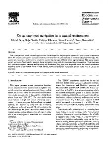
Fig. 2. Example l-precedence
ordering (2)-(3)-(l).
(19)
In equation (19) h, is the calculated steplength of module number i, provided by the integration routine. This method, unlike equation (17), requires any initial value of the time horizon. And, since it is not desirable to let the user specify an initial time horizon, equation (19) can at least be used for calculation of the initial time horizon. Implementation The user gives initial states for all modules. But the system will also be able to compute steady-state values, to be used as initial states in a dynamic simulation. Error tolerance and maximum order of polynomials are user-supplied variables. The system will also store all variables, when terminating, to make it possible to restart the simulation with other experimental conditions, if desirable. External disturbances are user-specified subroutine(s), which may be connected to any module. Disturbances may be physically derived models of the surroundings, or they may be empirical correlations. The surroundings may, for instance, be the pressure relief system, the ambient temperature or the procedure for starting up a pump. Disturbances will often create discontinuities in the unit model, and these are more likely to happen when a state variable has reached a certain threshold (state event), or at a certain time (time event). State events are determined by a user-supplied switching function, as illustrated in Fig. 1. They will be taken care of by letting the particular integration routine detect the discontinuity and locate the time. Then, the time horizon is reduced to match this time, and the sequence is recomputecl. To restart after a discontinuity has occurred, the same procedure will be used as proposed for multistep integration methods by Gear and Osterby [9].
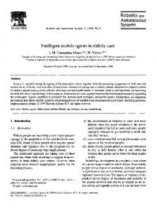
Fig. 3. Example 2-precedence UH3)-(2)-(W4).
stream. MT is a mixer with two input streams and one output stream. In addition, MT has the possibility of having an external disturbance, which is an extra input stream. The models, describing these units, are very simple with only two state variables each-see the Appendix. But the main point, here, is to illustrate two aspects of the approach-namely steplength and accuracy. Szephgth To illustrate the steplength control of the two solution methods, the number of function evaluations are compared in Table 1. This very clearly illustrates the savings in the number of function evaluations by using the proposed algorithm. Here, Euler’s method (embedded with the modified Euler’s method for estimation of local error) and the same integration tolerance (10m4) are supplied to all integrations, for the sake of comparison. Theoretically, the number of evaluations with the sequential approach will never exceed that of the simultaneous solution in any module, provided that the same integration method and tolerance are used.
RESULTS
The proposed algorithm is currently being tested, so every aspect of it is not yet fully investigated. Here, only two simple example problems are shown, where steplength control and accuracy are compared with the simultaneous solution of the equations.
ordering
Table
1. Number Module No. I
Example
I
2 3 SllFll
of function
evaluations
Simultaneous solution
Sequential solution
884 884 884
297 641 773
2652
1711
513 513 513 513 513
127 208 319 140 519
2565
1313
Problems These problems are constructed arbitrarily by means of two building blocks-SP and MT. SP and MT are types of modules and the number in parentheses corresponds to the module number. Here, SP is a splitter with two output streams and one input
Example
2
1 2 3 4 5 Sum
M.
384
HILLESTAD
and T.
module w.r.t. steplength up to time ~1.3, and from there, Module 3 is the restrictive one. From these two problems, which are not even stiff problems, it is obvious that there is a lot to be saved in the number of function evaluations. Even when using an initial integration steplength of 0.001, as illustrated, 3.5 and 49% savings are achieved from Examples 1 and 2, respectively. For stiff and large-scale problems the savings are expected to be much higher. This comparison is not quite fair as the overheads are not taken into account, but for large-scale problems the overheads will become relatively less significant [24]. The overheads will also be taken into account in the comparison, when larger and more realistic problems will be treated in a later study.
For Module 5 of Example 2 this is not quite true. This discrepancy stems from the fact that after every new time horizon, the initial steplength is set to an unnecessarily small value. But, although this can be avoided by simply remembering the last steplength from the previous time horizon, the extra evaluations, by doing this, are surprisingly few. Of course, we should use an initial steplength equal to the last estimate from the previous time horizon if that is possible with the routines available. The plots in Fig. 4 are steplength as a function of time for Example 1; only accepted steps are plotted, whereas, Table 1 includes both accepted and rejected steps (two evaluations per step). From the plots, in Fig. 4, it can be seen that Module 2 is the restrictive
1000
0
HERTZBERG
1
100 t
r
i._;
00011 o
’
1
’
2
’
3
’
4
’
’
5
’
6
7
I
I
I
6
9
10
Time
Fig. 4a. Integration steplength of the simultaneous solution of Example 1.
0 001
0
1
I
I
I
I
I
I
I
I
I
2
3
4
5
6
7
6
9
10
Time
Fig. 4b. Steplength of Module 1.
The sequential modular approach
2
3
-
4
5
6
385
7
8
9
10
Time
Fig. 4c. Steplength of Module 2
I
I
I
I
I
I
I
4
5
6
7
8
9
10
Time
Fig. 4d. Steplength
Accuracy By reducing the number of function evaluations we would expect accuracy to be reduced, but that is not the case. The saved evaluations are those not necessary to attain integration accuracy. However, the expected accuracy of the sequential method is not as high as that of the simultaneous solution because prediction is involved in the sequential method. Prediction may also be involved in the simultaneous solution, but the prediction is then done over a much shorter time interval. From the two examples shown here, there are no significant deviations between the solution trajectories of the two methods. The worst case, which is Module 2 of Example 1, is shown in Fig. 5. The
of Module
3.
deviation between the solutions of x2 is due to its strong dependency of x, when x, is small. Method 3, equations (12) and (13), is used for prediction of tear-stream variables for the two examples.
DISCUSSION
Perhaps, the greatest advantage of the independent modular approach is the multirate nature of the method. Slow units, like a flash tank, need few function evaluations over the time horizon, while fast units, like control units have to do several more evaluations to attain the same integration accuracy. The total number of function evaluations required is therefore reduced when compared to the simulta-
386
M.
;
HILLESTAD
and T.
HERTZBERG
1 o-
00
0
1
2
3
2
3
4
5
6
7
0
4
5
6
7
6
9
10
I
I
9
10
Time
Fig. 5. Solutions
of Module
2 of Example
1. Sequential solutions.
neous solution, as illustrated. This advantage is very attractive, when the function evaluations are laborious. This is often the case in process simulation with chemical unit operations involving heavy thermo-physical property estimations. However, the independent modular approach requires more administration, so increased program overheads should not override any savings. Small non-stiff problems, involving a few equations, will certainly not benefit from using this approach w.r.t. computer time. In general, a multirate method can only be competitive if one of two conditions is true; either the cost of function evaluation is high, or the system of equations is sparse (few interpolations). In large-scale process simulation, it is likely that both are true. For a modular system in general, and an independent modular system in particular, it is easier to do error debugging with respect to locating modelling or data errors. The software will be less complex and therefore easier to maintain. This is a well-known fact from steady-state simulation. Also, modelling or setting up new process configurations will be easier. By this approach it is possible to do “modelling in the large”, and the process engineer may test different control or process structures and designs within a short time. The independent modular approach makes it very easy to exchange integration routines with newer and better ones. We are not tied to one particular choice of integration method. It should also be mentioned, as an advantage of the independent modular approach, that it is even possible to use the analytical solution by integrating the model using the approxi-
modular
(........)
and
simultaneous
(-)
mative input polynomials. In addition, the integration routine does not even need to solve an initialvalue problem, but may equally well be solving a two-point boundary-value problem in time. One or several states may be design variables, which are to meet specified design requirements within a specified time. Another attractive aspect of the independent modular approach is that there is also great freedom w.r.t. choice of model type. Any module may use any type of model, provided that it is consistent with the rest of the module. Using a simultaneous solution, it seems to be difficult to combine differential equations with input-output models. By solving the modules simultaneously with a single integration routine, the integrator will solve a system of equations which also includes the algebraic interconnections. This is avoided when an independent modular approach is used. The total system of equations which is seen by the integration routines, will therefore be less complex than if all modules were solved simultaneously. The sequential modular approach is wellinvestigated, and a great deal of well-established theory and software exist for steady-state simulation. This may well be built upon for extension to dynamic simulation. Dynamic modules will have to be built, but with some modifications, the executive system will certainly suffice. Using the sequential modular approach in dynamic simulation, the tear-stream convergence problem will normally not be any problem at all. This is due to the capacities and dead times of process units, which act like filters to changes in tear variables. Convergence may only be a problem
387
The sequential modular approach when the time horizon is chosen to be greater than the time lag of a loop. Discontinuities have to be handled efficiently by a dynamic process simulator. Using the independent modular approach, the detection and localization of the time when the discontinuity occurs will be left to the particular integration routine. The time horizon will then be reduced to match the discontinuity point, and the integration is then restarted. When a discontinuity occurs, there is no point in representing the stream variables by polynomials interpolating points established before the discontinuity. The polynomial order has to be reduced according to Gear and Osterby [9]. They also propose how the new time horizon should be chosen when restarting after a discontinuity has occurred. By comparison of the sequential and parallel variants of the independent modular approach, it is obvious that the sequential approach involves less iteration variables and will therefore give a smaller error estimate of tear streams. Using the sequential approach, less work is involved in predicting tear variables for the same reason. The sequential variant will also be numerically more stable, because the sequential and the parallel approaches will correspond to Gauss-Seidel and Jacobi iteration, respectively. The sequential procedure has stability properties similar to an implicit integration, while the parallel procedure has stability properties similar to an explicit integration. The parallel approach may be computationally preferable only when using a multiprocessor computer where each module is computed on an individual processor-i.e. parallel processing. The sequential approach is limited by the assumption of directed information streams. When an information stream changes direction, the simulation will break down, unless the system automatically recovers by finding a new precedence ordering, tear streams and prediction modules. Unfortunately, the information streams are not always identical to mass and energy streams. Quite often, process units are affected by downstream units through the output pressure. This is handled by letting the output pressure become an input information stream to the actual module. The independent modular approach will impose an external error control in addition to the error control of the integrators. This is unwanted, but is a necessary part of the coordination algorithm. But, as already stated, by calculating the modules sequentially there will normally be no problem with convergence of tear streams. When compared to the simultaneous solution of equations, the accuracy will normally be poorer due to prediction of tear variables. But if predictions are accurate, the same accuracy may be attained with the proposed method. This was the case when running Examples 1 and 2 using prediction Method 3. Finally, the stability analysis for a multirate method, like the independent modular approach, is non-trivial. In fact, having merely two subsystems,
each with different step control, will involve complex methematics for finding the region of stability, as demonstrated by Gomm [15]. But since we are primarily interested in the region of stability for the time horizon, an analysis of the corresponding multistep integration method will suffice, assuming that the order of the integrators is at least p + 1 [4]. The internal integrator steplengths are controlled by the local error tolerance, and will therefore lie within their regions of stability. thank Professor S. P. Nsrsett of the Department of Numerical Mathematics for his help with the presentation and for his comments and suggestions Acknowledgement-We
during
the work. NOMENCLATURE
b, = Polynomial coefficients defined in equation (1) D = Pascal’s triangle matrix emar = Maximum error tolerance of tear variables, user supplied err = Absolute error of tear variables, calculated f,f, = State equations and the Jacobian g, g,, g,, g, = Output equations, and partial derivatives of g w.r.t. x, u and v h, = Steplength of module No. i L,, L, = Vectors from equation (6) p = Degree of interpolation polynomials IFP,= Matrix used in equation (14) 4 = Number of time intervals used in the interpolation procedure (q = p - 1) Q, = Matrix used in equation (15) r. = Vector used in equation (14) s, = Vector used in equation (15) I, = Discrete time T,, = Time horizon = t,+ , - t, U(I) = Exact input function u,(t), u,(f ) = Approximated input functions, polynomials of degree p and centralized at t,, scalar and vector u,, II, = Input value at t,, scalar and vector upt. u,, = Tear variables, predicted and calculated v(r) = External disturbance functions, user supplied x, = State vector at 1, y, = Output vector at I, Greek letters r,, /r’, = Coefficients in the predictor equation (12) ‘;, = Coefficients in the extrapolation equations (10) and (I I) TV, = Coefficients in the extrapolation equation (13) 6 = Difference calculated in equation (4) fi = Difference calculated in equation (5)
REFERENCES
I. I. T. Cameron, Lat. Am. J. them. Engng appl. Chem. 13, 215 (1983). Comput. them. Engng 1, 75 (1977). 2. V. Hlavacek, 3. J. G. Balchen, M. Fjeld and S. Selid, Paper presented at the A. AIChE Mtg, Washington, DC. (1983). (1980). 4. C. W. Gear, ReportUIUCDCS-R-80-1000 Numerical solution of differential5. I. T. Cameron, algebraic equations in process dynamics, Department of Chemical Engineering and Chemical Technology, Imperial College of Science and Technology, London (1981).
M. HILLESTAD and T. HERTZBERG
388
6. C. W. Gear and L. R. Petzold, Report UIUCDCS-R82-1103 (1982). 7. D. Ellison. Maths Comouf. Sitnularion XXIII. 12 (1981). 8. W. H. Eniight, K. R. jackson, S. P. Nsrset; and P. 6. Thomsen, Trans. math. Softw. In press. 9. C. W. Gear and 0. Osterby, Trans. math. Softw. 10, 23 (1984). 10. R. K. Wood, R. K. Thambynayagam, R. G. Noble and D. J. Sebastian, Simulation 36, 221 (1984). 11. S. Kuru and A. W. Westerberg, Comput. them. Engng 9, 175 (1985). 12. G. D. Hatchel and A. L. Sangiovanni-Vincenttelli, Proc. IEEE 69, 1264 (1981). 13. A. Orailogu, Report UIUCDCS-R-79-959 (1979). 14. J. F. Andrus, SIAM JI numer. Analysis 16, 606 (1979). 15. W. Gomm, Maths Compur. Simulation XXIII, 34 (1981). 16. S. Skelboe, Multirate Integration Methods. Elektronik Centralen, Hsrsholm, Denmark (1984). 17. G. Qderlind, Report TRITA-NA-8008, Royal Institute of Technology. Stockholm, Sweden (1980). 18. 0. A. Palusinski and J. V. Wait, Simulation 30, 85 (1978). 19. M. Hillestad, Thesis, Laboratory of Chemical Engineering, Norwegian Institute of Technology, Trondheim, Norway (1986). 20. J. Fagley and B. Carnahan, Proc. PAChEC-83, 3rd Pacific Chemical Engineering Conf.. Seoul, Korea, pp. 78-84 (1983). 21. G. K. Patterson and R. B. Rozsa, Comput. them. Engng 4, 1 (1980). 22. Y. C. Liu and C. B. Brosilow, Paper presented at the AlChE Diamond Jubilee Mig, Washington, D.C. (1983). 23. J. W. Ponton, Comput. them. Engng 7, 13 (1983). 24. L. G. Birta, Maths Comput. Simulation XXII, 189 (1980). 25. W. C. Gear, h’umerical Initial Value Problem in Ordinary Differential Equafions. Prentice-Hall, Englewood Cliffs, N.J. (1971). 26. W. J. Cook and C. B. Brosilow, Paper presented at the 73rd A. AZChE Mfg. Chicago, Ill. (1980). 27. A. Barrett and J. J.-Walsh, ?omput.‘chem’. Engng 3, 397 (1979). 28. T. Gundersen and T. Hertzberg, Model IdentiJication Confrol4, 139 (1983).
APPENDIX In both modules. MT and SP, the states x, and x2 are the level and concentration of the liquid in the tanks, respectively. The initial conditions and the parameters were chosen arbitrarily for the modules shown in Figs 2 and 3. The parameter vector p and the initial conditions are figures attached to the particular module number. Module MT Input
variables
u, = flow rate of Stream
1
u2 = concentration
of Stream
u, = flow rate of Stream
2
uq = flow rate of Stream
2
External
1
disturbances
u, =p3 = flow rate is constant v2 = p4 = concentration
is constant
State equations xi = (VI + u, + u, -pZfi)/p,; x; = [V,(% -x2)
x,(a)
+ u,(u* - x2) + UJ(U~-
Output
= -rjo
~2Mw2)~
.da) = -50
equations
Y, = pz fi
= flow rate
Y2 = x2
= concentration
Y; = O.5p,x;l& y; = x; Module SP Input
variables
u, = flow rate u2 = concentration State equations xi = [u, - (P2 fp,)
x; =bl(U2Output
d%I/~I;
%)II(PIx,);
x,(a) = xl0
x2(a) =x20
equations
y,,, = p2 &
= flow rate of Stream
Y1.2=x2
= concentration
flow rate of Stream
Y,,, =p,&= Y&2=
=
x2
concentration
1
of Stream 2
of Stream
Y;., = 0.5P2&lJj;l Yi.2=x; Yil = 0.5P,x;l&l Yi.2=x;.
Numerical values for Example I Module MT p, = p2= p3 = p4 = Xl0 = x20 =
10.0 1.2 1.2 0.03 0.5 0.02
1
Module SP
2
Module SP
3
p, = 1.0 p2 = 1.3 p, = 3.2
p, = 1.8 pz = 0.9 p, = 0.5
x,,=2.1 xzO= 0.09
xi0 = 4.6 x20 = 0.89