Proceedings of the ASME 2011 Dynamic Systems and Control Conference DSCC2011 October 31 - November 2, 2011, Arlington, VA, USA
DSCC2011-6169
DYNAMICS OF NETWORKS WITH STOCHASTICALLY SWITCHED CONNECTIONS Igor Belykh Department of Mathematics and Statistics Georgia State University Atlanta, Georgia 30303
[email protected]
Martin Hasler School of Computer and Communication Sciences Ecole Polytechnique Fédérale de Lausanne CH-1015 Lausanne, Switzerland
ABSTRACT
There are two time scales present in such systems, namely the time scale of the dynamical system itself and the time scale of stochastic switching. In this paper, we assume that the stochastic switching is much faster than the dynamical system. Hence, we expect the stochastically blinking system to behave like the averaged system where the dynamical law is simply averaged over the driving stochastic variables at each time instant. What this exactly means is a non-trivial problem and we believe to contribute substantially to its solution in this talk.
This talk discusses the influence of network structure on the dynamics of networks with fast on-off stochastic connections. It is investigated to what extent the trajectories of a stochastically switched (blinking) network follow the corresponding trajectories of its averaged analog where the stochastic connection are replaced with static ones. Four cases have to be distinguished, depending on whether or not the averaged system has a unique attractor and whether or not the attractors are invariant under the dynamics of the blinking system. The corresponding asymptotic behavior of the trajectories of the blinking system is described and illustrative examples are given.
MODEL OF BLINKING NETWORKS In many technological and biological networks, the individual nodes composing the network interact only sporadically via short on-off interactions. Packet switched networks such as the Internet are an important example. To model realistic networks with intermittent connections, we have introduced a class of dynamical networks with fast on-off connections that are called “blinking” networks [13]. These networks are composed of oscillatory dynamical systems, whether identical or different, with connections that switch on and off randomly, and the switching time is fast, with respect to the characteristic time of the individual node dynamics. The general “blinking” model reads
INTRODUCTION Networks of dynamical systems are common models for many systems in physics, engineering, chemistry, biology, and social sciences. Among the best known examples are Internet routers, genetic networks, ecological networks, neuronal networks, communication and social networks [1,2]. Recently, a great deal of attention has been paid to algebraic, statistical and graph theoretical properties of networks and their relationship to the dynamical properties (e.g., synchronizability and information transmission capacity) of the underlying network (see, for example, [1-16]). In most studies, network connectivity is assumed to be static. However, in many realistic engineering and biological networks the coupling strength and/or the connection topology can vary in time. Researchers are only now beginning to investigate the link between time-varying structure and the overall network dynamics [13-16].
dxi dt
n
1,..., n = Fi ( xi ( t ) ) + ∑ ε ij sij (t ) Pc x j , i = j =1
(1) 1 d where xi = ( xi ,..., xi ) is the d-vector of the coordinates of
the ith oscillator and function Fi ( xi (t )) defines the dynamics of the ith oscillator. The non-zero elements of the d × d projection matrix Pc determine which variables couple the
1
Copyright © 2011 by ASME
oscillators. The n × n connection matrix with constant
ε ij ≠ ε ji
graph as functions
)
chaotic dynamical systems. There are several important cases to distinguish, depending on whether or not the attractor in the averaged system is unique and whether or not it is shared by the blinking system for all switching sequences. We now address the question what happens when t → ∞ by presenting four different examples, each representing a different class of blinking systems.
defines the time-varying connection
sij (t )
dependence is described
(
G = ε ij sij (t )
depend on time. Their time-
as follows. The time axis is divided
into intervals of length τ intervals and sij (t ) are assumed to be binary signals that take the value 1 with probability p and the value 0 with probability 1-p in each time interval. More precisely, the probabilistic blinking model is the following. During each time interval of length τ every possible connection is turned on with probability p, independently of the switching on and off of the connections, and independently of whether or not it has been turned on during the previous time interval. It is worth noticing that this is the simplest stochastic switching model which can be generalized in different ways.
Example for Case 1: Synchronization in networks with a time-varying coupling We start off with a small-world-type network [1] which consists of a regular lattice of cells with constant 2K-nearest neighbor couplings and time-dependent on-off blinking couplings between any other pair of cells [13]. At each moment, the coupling structure corresponds to a small-world graph, but the shortcuts change from time interval to time interval (see Fig. 1).
In technology, practical systems exist that can be modeled rather precisely by the blinking model (1). Processes on the Internet may interact in order to achieve many different goals, but in order to be able to interact in a controlled way, they need to refer to a common time reference. In other words, the clocks that generate the local time for the computer need to be synchronized throughout the network. This is done by sending information about each other computer's time as packets through the network . The limiting factor in the time accuracy of the local computer is the stability of the local clock, which is usually implemented by an uncompensated quartz oscillator. The synchronizing signals, that aim at reducing the timing errors, should be sufficiently frequent in order to guarantee a sufficient precision of synchronization between the clocks, but the network should not be overloaded by these "administrative" messages. This is a trade-off between the precision of synchronization and the traffic load on the network. To some extent, this frequent "blinking" network administration is a way to provide reliable and precise functioning of the network composing of non-precise elements. FIGURE 1. THE BLINKING MODEL OF SHORTCUT CONNECTIONS. PROBABILITY OF SWITCHINGS P = 0.01, THE SWITCHING TIME STEP Τ = 0.1. THE BLINKING MODEL CONSISTS OF THE PRISTINE WORLD (THE REGULAR LOCALLY COUPLED LATTICE OF 30 OSCILLATORS WITH CONSTANT COUPLING COEFFICIENTS) AND A TIMEDEPENDENT ON–OFF COUPLING BETWEEN ANY OTHER
It is natural to expect that that if the connections in the blinking model (1) switch fast enough, i.e., if τ is sufficiently small, then a solution of the blinking system (1) follows closely the solution of the averaged deterministic system obtained from the blinking system by replacing the binary signals
sij (t )
with
constants p, where p is the switching probability. The fact that the rapidly switched system has the same behavior as the averaged system seems obvious, but in fact there are exceptions, and therefore, a careful proof of this property is needed which shows on what parameters the occurrence of the exceptions depends. While averaging is a classical technique in the study of nonlinear oscillators, averaging for blinking systems needs some special mathematical techniques for obtaining rigorous convergence proofs. Such techniques have been used in [13] for synchronization of blinking networks of
PAIR OF CELLS
ε sij (t )
(TOP PANEL).
AVERAGED
NETWORK: THE PRISTINE WORLD WITH THE LOCAL COUPLING STRENGTH AND THE ADDITIONAL GLOBAL COUPLING ε p . HERE, P IS SMALL, SUCH THAT THE WIDTH OF THE LINKS MAY BE THOUGHT OF AS THE COUPLING STRENGTH (A STRONG COUPLING WITHIN THE PRISTINE WORLD AND A WEAK COUPLING FOR THE REMAINING ALL-TO-ALL LINKS) (BOTTOM PANEL).
2
Copyright © 2011 by ASME
For simplicity, the connection matrix assumed to be symmetric
ε ij = ε ji
(
G = ε ij sij (t )
)
is
and have vanishing row-
sums. The latter requirement is a necessary condition for the existence of complete synchronization among the oscillators: x1 (t)= x2 (t)= … = xn (t). The question is how large the coupling constant ε and the probability p (for the presence of a link) have to be chosen in order to guarantee complete synchronization of the movement of the n oscillatory systems. It was rigorously proven in [13] that, for almost all switching sequences, the threshold for complete synchronization in the blinking model is the same as the threshold in the averaged model, where the remaining links are constant, with value pε (see Fig. 1(bottom panel)). In other words, the set of on-off shortcut switching sequences that fail to force total synchronization has probability zero. For this property to be true, necessarily the switching time τ must be much smaller than the characteristic synchronization time of the network. This allows the use of averaging. The proof that the synchronization solution of the blinking system closely follows that of the averaged system involves the construction of a Lyapunov function that decreases along solutions of the averaged and the blinking systems. Actually, because of the stochastic nature of switching, this is not always true in the blinking system. However, the Lyapunov function may increase temporarily, but the general tendency is to decrease. This can be expressed by showing that after a certain time ∆t the Lyapunov function decreases for almost all switching sequences. The synchronization threshold in the averaged system that also almost surely guarantees synchronization in the blinking model (Fig. 2) can be calculated by the Connection Graph Method [8] and equals
a L ε* ≅ ⋅ , n 1 + p( L − 1)
FIGURE 2. DEPENDENCE OF THE SYNCHRONIZATION THRESHOLDS ON THE PARAMETER P IN THE AVERAGED NETWORK AND ON THE PROBABILITY P OF THE SHORTCUT APPEARANCE IN THE BLINKING MODEL. THE PRISTINE WORLD IS A RING OF 30 2K-NEAREST NEIGHBOR COUPLED LORENZ SYSTEMS WITH STANDARD PARAMETERS. THE SWITCHING TIME IN THE BLINKING MODEL Τ = 0.1. THE ANALYTICAL CURVE
= ε * (a / n ) L /(1 + p( L − 1))
(SOLID LINE) FITS THE NUMERICAL DATA (SMALL CIRCLES) REMARKABLY WELL. THE BLINKING INTERACTIONS ARISING EVEN WITH A VERY SMALL PROBABILITY SIGNIFICANTLY LOWER THE SYNCHRONIZATION THRESHOLD. THE BLINKING EFFECT OF THE SHORTCUT APPEARANCE PROVIDES MORE RELIABLE GLOBAL COORDINATING PROPERTIES THAN THE NETWORKS WITH THE SMALL-WORLD BUT FIXED COUPLING STRUCTURE WHOSE PERFORMANCE STRONGLY DEPENDS ON THE PARTICULAR CHOICE OF THE SHORTCUTS.
where L=n/(2K) is the
average path length of the coupling graph corresponding to the pristine world, and a is the double coupling strength sufficient for synchronization of two mutually coupled systems.
It is important for the description of distinct types of blinking networks to emphasize that in this above case, the averaged system has a single attractor, namely the synchronization manifold x1 = x2 = …= xn. Furthermore, the attractor is also an invariant set for the blinking system, for any switching sequence. This allowed one to prove that for almost all switching sequences, the solutions of the blinking system converge to the attractor (i.e., synchronize in the example), if the switching period τ is short enough. The next example does not have this invariant subspace for the blinking system.
3
Copyright © 2011 by ASME
Example for Case 2: Switching power converter
around it (Fig. 4). The fluctuations diminish in size as the switching period τ decreases.
Consider the circuit of Fig. 3. Its function is to convert dc power at voltage E to dc power across the resistor R. The switch is usually operated periodically at rather high frequency.
i + E _
L C
+ v _
R
FIGURE 4. SOLUTION (CURRENT) OF THE AVERAGED (SMOOTH CURVE) AND OF THE BLINKING SYSTEM. PARAMETERS ARE E = 1, R = 4, L = 1.5, C = 0.4,
FIGIRUE 3.. SWITCHED BOOST POWER CONVERTER AS AN EXAMPLE OF A BLINKING NETWORK.
P = 0.5, Τ= 0.01.
This frequency and its harmonics are filtered as much as possible. However, some parasitic frequency components remain and pollute the network. Another possibility is to operate the switch stochastically. The advantage is that the power of the parasitic components is distributed over a whole frequency range and therefore it is less disturbing than the narrow band parasitics in the case of periodic switching.
In both examples discussed so far, the salient feature of the dynamics was the convergence to a unique attractor of the averaged system. In the next example the averaged system is multistable, i.e., there is more than one attractor. Example for Case 3: Coupled bistable systems Consider the system of two linearly coupled bistable systems:
Let the switching variable be s = 1 when the switch is closed and s = 0 when the switch is open. The circuit equations and the corresponding averaged equation are given, respectively
di E v = − (1 − s ( t ) ) dt L L dv i v 1 s (t )) − =− ( dt C RC η dξ E = − (1 − p ) dt L L dη ξ η =(1 − p ) − dt C RC
dx dt dy dt
(2)
= f ( x ) + 8s ( t )( y − x ) =
where
f (= x) (3)
2 f ( y ) + 8s ( t )( x − y )
(
x 1 − x2
(4)
)
and s(t) is a switching function as represented in the previous sections. Suppose that the switch is closed with probability p =
dx / dt 0.1. When x = 1, we get =
8s ( t )( y − 1) and thus
The averaged system is asymptotically stable. At the dx / dt ≤ 0 for x = 1, − 1 ≤ y ≤ 1 . With similar reasoning for equilibrium point, η = E/(1-p), i.e. the averaged dc-output x = -1, y = 1 and y = -1, we find that system (4) leaves the unit voltage is larger than the input voltage (this is the reason for square in the x-y-plane invariant. We consequently shall limit calling it a boost converter) and adjustable by choosing p. The our attention to the dynamics in the unit square. mechanism that keeps the solution of the blinking and the averaged system together is the convergence to the equilibrium The isolated bistable systems are described by point in the averaged system. Note that this equilibrium is not shared by the blinking system. In fact, when s = 0 (open dx dy switch), the system has a different asymptotically stable = = f ( x) and 2 f ( y) equilibrium point (v = E) and when s = 1 (closed switch), the dt dt solution grows linearly in time. The consequence is that the solution of the blinking system cannot converge to the They both have two stable equilibrium points x = 1 and x = -1, equilibrium point of the averaged system, but it fluctuates and an unstable equilibrium point x = 0.
4
Copyright © 2011 by ASME
When the switch is open (s(t) = 0), the two bistable systems do not interact and the combined system has 4 stable and 5 unstable equilibrium points, namely all combinations of x = -1, 0, 1 and y = -1, 0, 1. When the switch is closed, there remain only 2 stable (x = y = -1, 1) and 1 unstable equilibrium (x = y = 0) points. The same is true for the averaged system
The correct functioning of this network is the following. At time t = 0, the N given numbers are loaded as initial conditions xi(0), i = 1, …, N. Suppose that the largest among these numbers is xm(0). Then, the state vector x evolves in time according to (15) and converges to the equilibrium point x such that xm ≥ 1 and xi ≤ −1 for i ≠ m . In terms of the
dξ = dt dη = dt
for i ≠ m . Hence, the whole system must have N asymptotically stable equilibrium points, one for each value of m, the index of the state with the largest initial value. The state space is divided into the N basins of attraction of these equilibrium points.
f (ξ ) + 0.8 (η − ξ )
= ym outputs, this means
(5)
2 f (η ) + 0.8 (ξ − η )
It is not difficult to see, that it is not possible to a “winner-takeall” CNN with only local connections. On the other hand, local connections have an evident advantage when it comes to the realization of the CNN as an integrated circuit. A way out of this dilemma is to use switched instead as hardwired non-local connections and realize them by sending packets on a communication network that is associated with the CNN. Such a communication network has to be present anyway in order to charge the initial conditions and to read out the results.
The blinking system has the two stable equilibrium points in common with the averaged system. Therefore, the solution of the blinking system can actually converge to one of these equilibrium points, contrary to the switched power converter, where convergence to the equilibrium point of the averaged system was not possible. However, there is a small probability, that starting from the same initial state the solution of the blinking and the solution of the averaged system do not converge to the same equilibrium point. The faster the switching, and the farther away from the basin boundary of the equilibrium points, the smaller is this probability.
Thus, we consider the blinking system
dxi dt
Example for Case 4: Cellular neural network with shortcuts Consider a two-dimensional array of locally coupled first-order linear systems with a piecewise linear output function, known under the name of cellular neural networks (CNN). Such networks can perform many signal processing computations using their intrinsic nonlinear dynamics. One way to implement this is to insert data as initial values of the states and to let states converge to an equilibrium point of the (multistable) network. The mapping from the initial to the final states is the function performed by the network.
yi
=
α p
N
∑
j not nearest neighbor of i
N
∑
j nearest neighbor of i
yj +
sij (t ) y j + κ
f ( xi ) (7)
where in each time interval
( k − 1)τ ≤ t ≤ kτ
sij(t) is
constant, of value 1 with probability p and of value 0 with probability 1-p. Its corresponding averaged system is (6). As a numerical example, we consider a blinking 4 x 4 CNN (N = 16) that has the task to determine the largest among the 16 numbers
∑
f= ( xi )
= − xi + (1 − δ ) yi − α
+
However, certain functions cannot be obtained directly using only local connections. This is the case of the “winner-take-all” function, where the maximum among a given set of numbers has to be determined. The following globally coupled network of one-dimensional systems realizes this function for a suitable choice of the parameters α, δ and κ. N dxi = − xi + (1 − δ ) yi − α y j + κ dt j =1
yi =
f= ( xm ) 1 and yi = f ( xi ) = −1
(6) 1 for xi > 1 xi for − 1 ≤ xi ≤ 1 −1 for x < −1 i
5
Copyright © 2011 by ASME
0.3644
0.3958
0.1871
0.2898
-0.3945 0.0833 -0.6983
-0.2433 0.7200 0.7073
-0.0069 0.7995 0.6433
0.6359 0.3205 -0.3161
(8) In Fig. 5a, x(3,3)(t) and in Fig. 5b x(4,1)(t) are represented, for the blinking system, for the averaged system and for the averaged system with only local connections. The trajectory of the blinking system follows the trajectory of the averaged system and approaches the corresponding equilibrium point. The state x(3,3) it increases beyond the value 1, as it should, since the element (3,3) in (8) is the largest, whereas the state x(4,1) decreases below -1. Thus, both the averaged system with its allto-all connections and the blinking system with its fixed local and the switched non-local connections perform the “winnertake-all” function correctly for this example, whereas the averaged system without non-local connections is unable to do so.
(b) FIGURE 5. TRAJECTORY COMPONENT XI(T) FOR A 4×4 “WINNER-TAKE-ALL” BLINKING CNN, WITH
a= 1, δ == 1.11, κ −13.89, τ = 0.0001, p = 0.1
(IRREGULAR LINE), TOGETHER WITH THE TRAJECTORY COMPONENT OF THE AVERAGED SYSTEM (UPPER SMOOTH LINE) AND THE AVERAGED SYSTEM WITH ONLY LOCAL CONNECTIONS (LOWER SMOOTH LINE). (A) COMPONENT OF THE CELL (3,3) WHOSE INITIAL CONDITION HAS THE MAXIMAL VALUE. (B) COMPONENT OF THE CELL (4,1).
The peculiarity of this system is that it has several attractors (stable equilibrium points), but practically all the time, none of them is an equilibrium point of the blinking system. Therefore, the trajectory of the blinking system cannot converge to an equilibrium point of the averaged system, but it can only get close to it, as in the switched power converter. Furthermore, there is a non-zero probability that it will approach the wrong equilibrium point, as in the third example. There is even a nonzero probability that after having approached the correct equilibrium point it will escape towards another equilibrium point of the averaged system. However, this last probability is much smaller than an initial approach to the wrong equilibrium point, so that it can be neglected in practice. In addition, once the trajectory of the blinking system is sufficiently close to a stable equilibrium point of the averaged system, a decision is taken and the system is stopped.
(a)
CONCLUSIONS A trajectory of the blinking system follows closely for some time the trajectory of the average system with the same initial state if switching is fast with respect to the dynamics of the averaged system (roughly). In order to extend this property to all (positive) times, the averaged system needs to have an
6
Copyright © 2011 by ASME
attractor. Four cases have to be distinguished, depending on • whether or not the attractor is unique •
[4] Wu, C.W. and Chua, L.O., 1996. “On a conjecture regarding the synchronization in an array of linearly coupled dynamical systems”. IEEE Trans. Circuits Syst. I 43, pp. 161-165.
whether or not the attractor is an invariant set for the
blinking system, for all switching sequences. The trajectories of the blinking system have different qualitative behavior for different cases. This is summarized in Fig. 6.
[5] Albert, R. and Barabasi, A.-L., 2002. “Statistical mechanics of complex networks”. Rev. Mod. Phys., 74, pp. 47-100. [6] Kurths, J., Boccaletti, S. Grebogi, S. and Lai, Y.-C. (editors), 2003. “Focus issue: Control and Synchronization in Chaotic Dynamical Systems”, Chaos, 13 [7] Boccaletti, S. and Pecora, L.M., 2006. “Focus issue: Stability and Pattern Formation in Dynamics on Networks”, Chaos, 16. [8] Belykh, V., Belykh, I. and Hasler, M, 2004. “Connection graph stability method for synchronized coupled chaotic systems”, Physica D , 195, pp. 159-187. [9] Belykh, I., Hasler, M., Lauret, M. and Nijmeijer, H., 2005. “Synchronization and graph topology”, Int. Journal of Bifurcation and Chaos, 15, pp. 3423–3433.
FIGURE 6. QUALITATIVE BEHAVIOR OF THE BLINKING SYSTEM IN THE FOUR CASES. UPPER PANEL: TRAJECTORIS CONVERGE TO THE SAME ATTRACTOR AS THE AVERAGED SYSTEM. LOWER PANEL: TRAJECTORIES REACH A NEIGHBORHOOD OF THE SAME ATTRACTOR AS THE AVERAGED SYSTEM. LEFT PANEL: PROPERTY HOLDS ALMOST SURELY. RIGHT PANEL: PROPERTY HOLDS WITH HIGH PROBABILITY.
[10] Barahona, M. and Pecora, L.M., 2002. “Synchronization in small-world systems”. Phys. Rev. Lett., 89, 054101. [11] Nishikawa, T., Motter, A.E., Lai, Y.-C. and Hoppensteadt, F.C., 2003. “Heterogeneity in oscillator networks: are smaller worlds easier to synchronize?”. Phys. Rev. Lett., 91, 014101.
Let us remark that all the above statements can be proved and explicit bounds can be given for the upper limit of the switching period as well as for the size of the neighborhood of the attractors. This has been done for case 1, specialized to synchronization, in [13] and for case 4 in [14]. The generalization to all cases constitutes the main research component of this talk.
[12] Newman, M. E. J., 2003. “The structure and function of complex networks”, SIAM Review, 45, pp. 167-256 (2003). [13] Belykh, I., Belykh, V. and Hasler, M., 2004. “Blinking model and synchronization in small-world networks with a time-varying coupling”, Physica D, 195, pp. 188-206.
ACKNOWLEDGMENTS
[14] Hasler, M. and Belykh, I.., 2005. “Blinking long-range connections increase the functionality of locally connected networks”, IEICE Transactions on Fundamentals E88-A, 10, pp. 2647-2655.
This work was supported by the National Science Foundation under Grant DMS-1009744. REFERENCES
[15] Porfiri, M.M., Stilwell, D.J, Bollt, E.M., Skufca, J.D., 2006. “Random Talk: Random Walk and Synchronizability in a Moving Neighborhood Network”, Physica D 224, pp. 102-113.
[1] Strogatz, S.H., 2001. “Exploring complex networks”. Nature, 410, 268-276. [2] Barabási, A. -L. and Albert, R, 1999. “Emergence of scaling in random networks”. Science, 286, pp. 509–512.
[16] De Lellis, P., di Bernardo, M., Garofalo, F., Porfiri, M., 2010. “Evolution of complex networks via edge snapping”, IEEE Transactions on Circuits and Systems I, 57(8), pp. 2132-2143.
[3] Pecora, L.M. and Carroll, T.L., 1998. “Master stability function for synchronized coupled systems”. Phys. Rev. Lett., 80, pp. 2109-2112.
7
Copyright © 2011 by ASME