Edge segmentation by Alternating Vector Field Convolution Snakes

IJCSNS International Journal of Computer Science and Network Security, VOL.9 No.8, August 2009

123

Edge segmentation by Alternating Vector Field Convolution Snakes Christian Roga߆, Sibylle Itzerott†, Bernd Uwe Schneider††, Hermann Kaufmann† and Reinhard F. Hüttl†† †

Remote Sensing Section, Helmholtz Centre Potsdam GFZ German Research Centre for Geosciences, Telegrafenberg, D-14473 Potsdam, Germany †† Scientific Executive Board, Helmholtz Centre Potsdam GFZ German Research Centre for Geosciences, Telegrafenberg, D-14473 Potsdam, Germany

Summary Active contours or snakes represent widely used methods in edge segmentation. Different, closed snake approaches have been proposed in the past but commonly lack of adequate capture ability and quality, noise robustness and convergence speed. In this paper a new closed approach namely “Alternating Vector Field Convolution (AVFC)” as well as a new force called “Yukawa Alternating Vector Field Convolution (YAVFC)” are proposed which minimize specific snake problems and enhance convergence speed. The comparison of both Gradient Vector Flow and Vector Field Convolution snakes with AVFC and YAVFC snakes determines the advantages of the new closed approaches.

Key words: Active contour, Snake, External force, Yukawa, Alternating vector field convolution

1. Introduction The segmentation of images by the extraction of edges can be considered as one of the main tasks in image processing. Assuming an image as a representation of its intensity function local extrema are generally searched to delineate differing elements. Many different methods of edge segmentation are proposed in literature. Active contours also known as snakes belong to modern methods in edge segmentation. In the case of parametric active contours specific parametric curves iteratively move through the image domain until certain mathematic conditions are fulfilled. The most basic condition is the minimization of a specific energy functional which finally contains two terms – the internal energy term and the external energy term. The internal energy term corresponds to the curve itself and controls the elasticity and the rigidity of the curve. The external energy term corresponds to the considered domain and is usually constructed as the potential of the domain. The solution of the minimization problem of the specific energy functional results in a force balance equation, where internal forces representing the internal term are at equilibrium with external forces Manuscript received August 5, 2009 Manuscript revised August 20, 2009

representing the external energy term. Typical approaches to model the external force are given by Balloon Forces, Gradient Vector Flow and Vector Field Convolution. These approaches address more or less the usual problems of snakes to capture boundary concavities, to overcome remaining image noise and to increase the convergence speed. In most cases they depend on nearby localization of initial contours towards the regions of interest, on a complex and case related determination of snake parameters and the amount of time given for the iterations. These properties do not distort the segmentation process unless similar images are used. For rapid segmentation and interpretation of different samples an extended approach based on the adaption of Vector Field Convolution and Balloon Snakes, Multi Resolution Analysis and alternating snake terms is proposed in this paper. They are called Alternating Vector Field Convolution Snakes (AVFC) respecting the underlying idea of Vector Field Convolution. Additionally a completely new force called Strong Force or Yukawa Force is implemented to cope with prior given general requirements of image segmentation. The related snake is called Yukawa Alternating Vector Field Convolution (YAVFC) snake. Both snake approaches proposed here are evidently able to enhance capture quality by simultaneously increased convergence speed.

2. Materials and methods 2.1. Traditional Snakes In [1,2,3] an active contour or snake is represented in two dimensions by a planar parametric curve v(s) = [x(s),y(s)]T, s Є [0,1] which moves through the spatial domain of an image to minimize the energy functional 11

∂v 2

∂2v

2

E = 0 (α + β 2 ) + Eext (v(s)) ds (1) 2 ∂s ∂s where α and β are weights to control the smoothness and ∂v

∂2v

the rigidity of the snake. and 2 refer to the first and ∂s ∂s second derivative of v with respect to s.

124

IJCSNS International Journal of Computer Science and Network Security, VOL.9 No.8, August 2009

Eext denotes the external energy function and is directly derived from the image. This function becomes small at the regions of interest (ROI), for instance at edges. Taken I(x,y) as the intensity function of an image typical external energy functions are (1) Eext (x, y) = − ∇I(x,y) 𝟐 (2) 2 𝟐 Eext (x, y) = − ∇(Gσ x,y ⨂I(x,y)) (3) where Gσ x,y is the 2D Gaussian function with standard deviation σ, ∇ denotes the gradient or Nabla operator and ⨂ represents the linear convolution operator [3]. Minimizing Eext the snake must satisfy the Euler equation ∂2 v

∂4v

α 2 + β 4 − ∇ Eext (v) = 0 (4) ∂s ∂s which is typically considered as a force balance equation 𝐅int (v) = −𝐅ext (v) (5) where the internal force 𝐅int (v) (5) represents α ∂4v

∂2 v ∂s 2

+

β 4 (4) and controls the smoothness and the rigidity of ∂s the snake. There, the smoothness parameter α acts like an elastic membrane and the rigidity parameter β as a thin plate [4]. The external force 𝐅ext (v) (5) deforms the snake towards the ROI. To solve equation (4), the snake is considered dynamically by treating v(s) as a function of time t → v(s, t). In [3] a solution is obtained when solving the gradient descent equation ∂2 v

∂4v

∂v

α 2 + β 4 + 𝐅ext (v) = (6) ∂s ∂s ∂t starting from the initial contour v(s, t = 0). A numerical solution to (6) can be achieved by using discrete s in a finite difference approach [3]. If the derivatives are approximated with finite differences and 𝐅ext (v(s, t)) expressed as [ 𝐅x (v(s, t)), 𝐅y (v(s, t)) ]T, the Euler equations can then be written for all snake elements as 𝐀𝐱 + 𝐅x (v) = 0 (7) 𝐀𝐲 + 𝐅y (v) = 0 (8) where A is a pentadiagonal banded Matrix. Assuming 𝐅ext (v(s, t)) constant at each iteration and time step and defining an iterative step size γ the resulting Euler equation is given by ∂v 𝐀v + 𝐅ext (v) = −γ (9) ∂v

∂v

∂t

If is discretised to = v s, t − v s, t − 1 = vt − ∂t ∂t vt-1 , then the snake elements or snaxels can be given by the dynamic equation vt = 𝐀 + 𝛄I

−𝟏

𝛄vt-1 − 𝐅𝐞𝐱𝐭 (vt-1 )

(10)

The parameter γ can also be considered as viscosity parameter and makes the snake harder to deform. Other approaches to solve the Euler equations are for instance the Finite-Element-Method [4] and the dynamic programming method [5].

2.2. Balloon Snakes According to [6] the closed, traditional snake has a low capture range if edges are not close enough to the initial contour and the snake tends to shrink in itself if the contour is not subjected to any counterbalancing forces. This property is strongly related to the choice of the parameter γ which directly influences capture range and speed. The balloon model increases the capture capability and speed by normalising the external force and extending it to 𝐅 (v) 𝐅ext (v) = k1 𝐧(v) − k ext (11) 𝐅ext (v)

where 𝐧 is the unit vector perpendicular to the curve, k1 is the amplitude of the force and k is the substituted time step [6]. The first term of (11) inflates or deflates the snake like a balloon depending on the choice of k1. The second term of (11) provides constant curve evolving speed depending on the choice of k. According to [1] closed balloon snakes may not move into boundary concavities depending on the set of k1 if they are inflated or deflated in the wrong direction as only the magnitudes of the forces are changed and not the directions.

2.3. Gradient Vector Field Snakes To enhance capture capability for distant edges and boundary concavities, [7] proposes a new external force formulation called Gradient Vector Flow (GVF) field and the respective snake GVF-snake. The external force 𝐅ext (v) is substituted by defining GVF field as a field v(x,y) = [u(x,y),v(x,y)] that minimizes the energy functional ℇ=

∂u

∂u

∂v

∂v

∂x

∂y

∂x

∂y

μ ( )2 + ( )2 + ( )2 + ( )2 + ∇f2v - ∇f2dxdy

(12)

where ∇f is the gradient of an edge map f, μ is a noise related regularisation parameter and ∂v 2 ∂y

∂u 2 ∂x

+

∂u 2 ∂y

+

∂v 2 ∂x

+

is the squared magnitude of the gradient of the optical

flow velocity according to [8]. If ∇f gets nearly homogenous regions or distant from optical flow term dominates the integrand smooth field and vice versa. The GVF field can be found by solving equations μ Δ v − ∇f 2 v - ∇f = 0

smaller in edges, the yielding a

where Δ denotes the Laplace operator with Δ =

the Euler (13) ∂2 ∂x 2

+

∂2 ∂y 2

in the 2D case. Equations (12) and (13) can be solved by treating u and v as functions of time and solving the generalized diffusion equation ∂v μ Δ v − ∇f 2 v - ∇f = 0 = (14) ∂t

IJCSNS International Journal of Computer Science and Network Security, VOL.9 No.8, August 2009

With regard to [9] forcing the snake into long indentations is still difficult. This is caused by excessive smoothing of the fields near the boundaries with respect to μ. As an extended approach for GVF-snakes to overcome the indentations problem the Generalized Gradient Vector Flow (GGVF) were proposed where both μ and ∇f 2 were substituted to g( ∇f ) and h( ∇f ) in the following equations ∂v g( ∇f ) Δ v − h( ∇f ) v - ∇f = (15) ∂t

− ∇f K

g( ∇f ) = e (16) h ∇f = 1 − g( ∇f ) (17) where K determines the degree of trade-off between field smoothness and gradient conformity [9]. g(∙) is a weighting function for a smoothly varying vector field. h ∙ is a weighting function which balances the data related ∇f .

2.4. Vector Field Convolution Snakes In accordance to [2,9] the GGVF-snake improves the ability to capture narrow boundary concavities, but is still sensitive to its parameters and to impulse noise and lacks of computational cost. In [2] a new edge-based static external force is proposed called Vector Field Convolution (VFC). The basic idea behind VFC-snakes is to convolve a specific vector field kernel with the edge map derived from the image, whereas the vector field strongly forces the snake towards the edges. The vector field kernel 𝐤(v) is defined by the equation 𝐤(v) = mn (v)

-v v

(18)

where mn (v) is the vector magnitude function of the vector at (x,y) and

-v v

is the unit vector pointing to the

kernel origin at (0,0) as the centre of the kernel. The magnitude function incorporates the distance from the origin and decreases the influence of edges if the edge elements are further away. This property is fulfilled by the given equations m1 v = ( v + ε)−γ (19) 2 −v ( 2 ) δ

m2 v = e (20) where γ and δ are used to control the decrease of ROI influence and ε denotes a small positive constant to prevent division by zero at the origin [2]. The VFC external force is computed by convolving the edge map with the vector field kernel given by the equation 𝐅vfc = f v ⨂ 𝐤(v) (21) where f v is the edge map. To support also the detection of weak edges, a mixed VFC-field was proposed by [2] given by the equation

𝐅ext (v) = 𝐅mix (v) =

125

∇𝐟, ∇𝐟 > 𝜙

(22) 𝐅vfc , ∇𝐟 ≤ 𝜙 where ϕ is a smoothing parameter like μ of GVF and ∇𝐟 denotes the gradient of an edge map. As a result the mixed VFC-field can be considered as the standard external force mixed with the VFC-field in homogenous regions depending on ϕ.

3. Extending the capture abilities and speed of VFC-snakes 3.1. The new Alternating Convolution Snakes (AVFC)

Vector

Field

With regard to [2], the VFC-snakes have better capture capabilities, are more robust to noise, are flexible when tailoring the force field and concurrently reduce computational cost for approximating the desired ROI. For the examples published in literature this assumption should be supported. But also in some specific cases for instance approximating a simple circle starting from inside the circle balloon snakes converge faster with the ROI. This follows from increased computational cost if large images are convolved with the filter kernel (21) independent of the method used for convolving the image. According to [10], where GVF-snakes are extended with specific balloon forces to increase convergence speed, an extended approach for VFC-snakes is contributed in the following. The convergence speed of snakes at the beginning of an iterative computation is dependent on the magnitudes of the vector fields used and is usually rather low. This could be improved by applying additional balloon forces on VFC-snakes, which concurrently restricts the snake approach to a closed loop. To avoid distortions of the VFC curve evolution, it is important to dynamically adjust the balloon extension with regard to the current deform iteration which gives the following equation for the snaxels based on (10) to vt = 𝐀 + γI

−𝟏

γvt-1 +

k1 i

𝐧(𝐯) − k

𝐅mix (𝐯) 𝐅mix (𝐯)

(23)

Depending on the choice of k1 the snake can be now inflated or deflated with respect to both the current deform iteration i and snake iteration t and, consequently, may simultaneously converge faster. The choice of k1 in equation (23) directly influences the behavior of the snake and always requires an user interaction. This is an undesirable property if the edge detection method is to work automatically. The decision on whether the snake needs to be inflated starting from the inner image centre towards the edges or deflated vice versa is also complex. To minimize the decision process, the use of Multi Resolution Analysis (MRA) and an alternating balloon force is suggested.

126

IJCSNS International Journal of Computer Science and Network Security, VOL.9 No.8, August 2009

To prevent balloon forces producing unpredictable results [11], the snake should be inflated in the first and coarsest resolution starting from the centre to extract the inner shape. In the next resolution level the snake should start from the previous snake curve and then be deflated towards the image centre and so on. This alternating approach concurrently respects possible shifts of real edges caused by resampling methods within the MRA and increases the speed of the whole edge detection process [12]. Defining resj with j Є [0,N] as the square root of the image size respecting MRA level j where 0 denotes the highest level and N the lowest level considered as the original image the equation (23) changes to vt,j = 𝐀𝐣 + γ𝐈𝐣

−𝟏

γvt-1,j +

−1 j k 1 res 0 res j

ij

k 𝐅mixj(𝐯)𝐅mixj(𝐯)

(24)

then gives the equation for the extended and mixed VFCsnake and is addressed as Alternating Vector Field Convolution Snakes (AVFC). The related equation is given to: 𝟏 γ

k

−1 j k 1 res 0 res j 𝐅mix j (𝐯) 𝐅mix j (𝐯)

ij

)

According to [2] the capture capability of a snake algorithm depends on the magnitude functions given by equations (19) and (20). As the basic property of the magnitude functions is to strongly decrease the magnitude with respect to the distance to the centre, any function which fulfills this requirement can be used. This is also fulfilled by the distance function based on the famous Yukawa Potential [13], which is related to the forces in equal charged particles. Those forces well-known as Strong Forces belong to the elementary forces considered in Nuclear Physics. As a special case of the Yukawa Potential the magnitude function

𝐧j (𝐯) −

Thus, the edge detection speed in the original image resolution increases by the initial contour estimation gathered from higher MRA-levels. This property is essential for large images. To avoid computation time intensive inversion of matrix 𝐀 + γI which size depends on the number of snaxels, [12] proposed a method to subdivide this matrix into 4 pieces. The solution for all pieces can be computed by using an optimized Cholesky decomposition. The speed limitation to this approach is the use of for-loops which slow the edge detection process for large images and can concurrently override available computer memory unless for-loops are usually consecutively saved in local memory. Based on [6] the inversion of matrix 𝐀 + γI can be completely avoided. 𝐀vt is approximated by 𝐀vt-1 which

vt,j = − ((𝐀 𝐣 + γ𝐈𝐣 )vt-1,j +

3.2. The new Yukawa Alternating Vector Field Convolution Snakes (YAVFC)

𝐧j (𝐯) − (25)

The AVFC can be imagined as a slowly growing and pulsating figure in 2D or bubble in 3D which delineates the region of interests. Curve evolving properties such as curvature, stiffness etc. can also be considered and will lead to parameterizations of e.g. α with respect to time t and resj .

mYuk v =

e− p v

(26)

v + ε1

fulfils the requirements for a force field to move free particles towards the edges where p is a small geometry factor and ε1 is a small, positive constant to prevent division by zero at the origin. Substituting the vector field kernel based on the equations (19 or 20) with equation (26) gives a new external force called Strong Force or Yukawa Force. The related Active Contour is addressed as Yukawa Alternating Vector Field Convolution Snake (YAVFC), belongs to the AVFC snakes and is based on the equation 𝟏

vt,j = − ((𝐀𝐣 + γ𝐈𝐣 )vt-1,j +

−1 j k 1 res 0

γ

res j

ij

fj v ⨂

-v 𝟐 v e p v + ε2

fj v ⨂

-v 𝟐 v e p v + ε2

k

𝐧j (𝐯) −

)

(27)

where ε2 is a small, positive constant to prevent division by zero at the origin. Concerning the property of the VFC external force to be a vector field with a negative divergence or a sink which is the underlying idea of VFCsnakes to force free particles towards the edges, this principle is similar for the YAVFC-snakes. With regard to the associativity and differentiation rules for partial derivatives of the convolution the divergence of YAVFC external force 𝐅YAVFC v is given by the following equation ∇ FYAVFC - fj v 𝟐

vj e

p vj

+ ε2

j

v = ∇

⨂ ∇ vj =

fj v ⨂

- vj 𝟐

vj e - f j vj 𝟐

vj e

p vj

tr I

p vj + ε2

= (28)

+ ε2

where ∇ denotes the divergence, ⨂ the convolution, fj v the MRA edge map and tr 𝐈 the trace of a dimension

IJCSNS International Journal of Computer Science and Network Security, VOL.9 No.8, August 2009

related identity matrix. Assuming non negative values for the edge map fj v , this new external force fulfils the basic requirements of being a sink for edges. With regard to (28) it is also possible to increase the influence of weak edges by multiplying the edge map with non-linear platykurtic, intensity related functions or to increase the influence of strong edges by multiplying the edge map with non-linear leptokurtic, intensity related functions. The direct use of the Yukawa Force (26) by multiplying with the gradient of an edge map can be considered as another approach to enhance the edge detection algorithms based on usual snake methods.

3.3. Noise removal In specific cases remaining impulse noise still distorts the edge detection and should be removed. Usually, a linear filter, for instance a Gaussian Filter or a non-linear filter, for instance the Median Filter is applied on the image to reduce remaining noise. The linear filter class reduces noise, but the blurring and smoothing of the edges can hinder the precise localization of edges if the edges are rather thin. The non-linear filter class reduces noise better, but shifts the edges somehow depending on the edge itself and the filter width. Those properties are quite complex to model and even not useful for an effective edge detection method based on snakes. Another way to minimize noise in images is proposed in [14,15]. Based on [14,15] adaptive, data-driven Coiflet hard-thresholds are applied on the image with respect to the BayesShrink rules. By [16] this method shall not distort edges, shall not produce grainier filter results and seems to be suitable for image denoising.

3.4. Edge map In [2] an edge map of a gray-level image is computed e.g. as the negative, squared norm of a Gaussian filtered image (3) or as inverse of the intensity function (2) for 1-Bitimages. The edge map is widely used as input for the most snake approaches. With regard to [17,18,19] a good edge detector must detect and localize edges and shall only allow single edge responses. These properties are given by the Canny edge detection method [17,19] and therefore, this method was applied to compute an edge map of an image. In some specific cases the canny filter tended to overestimate heterogeneous image regions as edges across a real edge depending on the choice of the hysteresis thresholds and the noise parameter σ. Reasoned by this property morphological dilations with small, rectangular discs as structuring elements were applied. The dilation

127

closes small gaps along and across the edges with respect to the disc size [20].

3.5. Speed issues [12] propose specific approaches to speed up snakes by, for example parallelization of computing processes, MRA and specific decompositions to invert the pentadiagonal matrix 𝐀 + γI . [2] suggests to use the Fast Fourier Transform (FFT) for the convolution of the VFC filter kernel with the edge map instead of linear convolution. Extending this approach it is possible to generally substitute discrete linear convolution with FFT in all snake methods [21]. This can also increase the computing speed of gradients, edge maps etc. Reducing the calculation time is essential for e.g. motion tracking, so it is also important to break the snake deformations and iterations if a certain threshold has been reached. Such a threshold is usually related to the difference or rate of change between the i-th and the (i-1)-th deformation or iteration. Setting ∆vt = vt − vt-1 as the difference between the deformation results in the following equation for an reliable threshold to T T ≥ threshold, continue ∆vt T [diag I , diag I ] (29) < 𝑡ℎ𝑟𝑒𝑠ℎ𝑜𝑙𝑑, 𝑏𝑟𝑒𝑎𝑘 Equation (29) can also be used when iterating each snake, not only when deforming it. The prior equation is similar to the convergence criterion proposed by [1] which is related to the Courant-Friedrichs-Lewy step-size restriction depending on the threshold chosen e.g. in (29). Another method to define the threshold for the iterations is the use of the change rate of the surrounded polygonal area by the snake. If the number of snaxels do not change significantly within the iterations, it is also not necessary to compute matrix 𝐀 + γI (25, 27) again, because it has not changed.

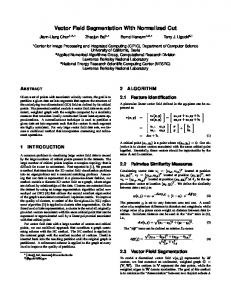
4. Results 4.1. Quality To test and to evaluate different snake approaches, 8-Bit rectangular, real and artificial sample images with different image sizes were chosen. Sample 1 was a 128 x 128 pixel sized part of a remotely sensed image (Fig. 1 a). Sample 2 and 5 were 256 x 256 pixel sized form primitives (Fig. 1 b and e). Sample 3 was a 64 x 64 pixel sized part of a remotely sensed image (Fig. 1 c). Sample 4 was a 128 x 128 pixel sized magnetic resonance image of the left ventricle of a human heart (Fig. 1 d).

IJCSNS International Journal of Computer Science and Network Security, VOL.9 No.8, August 2009

a)

b)

c)

d)

e)

f)

g)

h)

i)

j)

m)

n)

o)

k)

l) Fig. 1

128

Sample images (a-e), edge maps (f-j), gradient fields of classic and Balloon snakes (k-o)

At first all images were Coiflet based BayesShrink hardthresholded to reduce noise. Subsequent to the image denoising the edge maps were computed by applying the canny algorithm (Fig. 1 f-j). To remove small junctions and gaps in near to strong edges, morphological dilations with 2x2 rectangular discs as structuring elements were applied on the edge maps. In a next step remaining impulse noise was minimized by convolving the edge maps with a linear 2D-Gaussian filter kernel. To enable mixed external force fields (22), the gradients of the edge maps were additionally computed (Fig. 1 k-o). Then, small, centered circles were used as initial contours for different snake algorithms in different images (Fig. 2 a-e) which is similar to the initializations published in

literature. Starting from initial contours each snake was deformed 5 times within 500 iterations with the same parameter sets to ensure comparability. The external forces of the different snake approaches were computed in relation to their corresponding snake equations given before. According to [2] classic and Balloon snakes need sometimes initial contours relatively near the target contour to converge. This property was also observed and hence, they were not compared, as these approaches had to have other initial conditions such as GVF-snakes or did not converge based on the given initial contour in time. It follows from this that the GVF, the VFC, the AVFC and the YAVFC snakes were compared (Fig. 2).

IJCSNS International Journal of Computer Science and Network Security, VOL.9 No.8, August 2009

a)

b)

c)

d)

e)

f)

g)

h)

i)

j)

k)

l)

m)

n)

o)

p)

q)

r)

s)

t)

u)

v)

w)

x)

y)

Fig. 2

129

Initial contours on false colour sample images (a-e), results of GVF-snake (f-j), results of VFC-snake(k-o), results of AVFC-snake (p-t), results of YAVFC-snake(u-y)

With regard to the results given in (Fig. 2 f-j), the GVFsnakes were not able to converge completely with simple figures (Fig.2 g and j) conditioned by the amount of iterations used. This was also shown by [2] and can be supported. It’s also noticeable, that GVF-snakes tend to overestimate weak edges (Fig. 2 f,h,i) and hence, despite their smoothing abilities the GVF snakes in the original formulation may only have specific use.

VFC-snakes (Fig. 2 k-o) contribute better results in comparison to GVF-snakes with regard to given form primitives (Fig. 2 l and o) and enhance edge detection in specific samples (Fig. 2 k). Conditioned by the amount of iterations, VFC-snakes expand and move faster into concavities (Fig. 2 o) or in general towards boundaries (Fig. 2 m and n). They are flexible in usage and can be better adjusted than GVF-snakes. Therefore, they are

130

IJCSNS International Journal of Computer Science and Network Security, VOL.9 No.8, August 2009

4.2. Speed useful in a broader environment, but have to be finely adjusted. In relation to the results (Fig. 2 p-y) AVFC- and YAVFC snakes provided the best results and were able to capture all ROI independent of the given samples. This is caused for both the AVFC- and the YAVFC-snakes by the oscillations of parameters and different forces, but also conditioned by the Multi Resolution Analysis approach. Comparing the AVFC- with the YAVFC-snake, it can be assumed that the YAVFC-snake is more dependent on parameterizations, but produces smoother results and tends to move the snake more towards strong edges compared to the AVFC-snake. In contradiction to the YAVFC snake the AVFC-snake provides better results with regard to edges near the ROI. Concerning those results and the overall capture quality, the use of the new AVFC-snake and its derivative YAVFC-snake based on a completely new Force called Strong or Yukawa Force is suggestible for a broader range of applications.

To enable a broad range of applications, the convergence speed must also be considered. This is also a quality criterion. In relation to given samples AVFC and YAVFC snakes converge much faster on average (10 trials per sample) than GVF- and VFC-snakes (Table 1). This property is strongly related to the size of the image i.e. the scalar field. In some specific cases YAVFC-snake outperforms the AVFC-snake. For small image sizes VFC-snakes are also very fast, which is conditioned by the amount of computations in relation to YAVFC and AVFC snakes. This advantage is relevant until images are very small. In summary, AVFC and YAVFC snakes are more than 400 times faster than GVF and VFC-snakes and should be applied for most edge detection cases. This benefit will be enforced with increasing image size.

Table 1: Runtime for different Active Contour approaches

Sample 1 on average in seconds

Sample 2 on average in seconds

Sample 3 on average in seconds

Sample 4 average seconds

on in

Sample 5 in on average seconds

Total average time consumption in seconds

Rectangular 128 256 64 128 256 sample size GVF 76.5 350.2 18.1 92.9 399.9 937.5 VFC 98.6 592.5 1.1 67.4 523.9 1283.5 AVFC 0.4 0.61 0.5 0.3 2.3 0.3 YAVFC 0.1 0.59 0.4 0.6 0.3 2 *all results were achieved on a Intel Core2Duo L7500 X61s ThinkPad with 4 GB RAM within MS Windows Vista X64 Business and Interactive Data Language (IDL) 6.4 x64

With regard to the suggestion of [2] to use complex FFT for the convolution instead of discrete convolution, it is also necessary to test the proposed speed and to compare it.

To compare linear convolution with FFT convolution, averaged trials (100 trials for each case) for different matrix and kernel sizes were computed with regard to the convolution method (Table 2).

Table 2: Runtime for different convolution approaches

Matrix – size in both directions

Kernel – size in both directions

Linear convolution on average in seconds 0.0166 0.2520 3.9351 0.0395 0.6247 10.1722

FFT convolution on average in seconds 0.0003 0.0008 0.0033 Not measureable 0.0002 0.0003

Ratio - FFT / Linear on average

32 32 60 64 64 300 128 128 1300 128 3 Not measureable 256 3 3000 512 3 32485 *all results were achieved on a Intel Core2Duo L7500 X61s ThinkPad with 4 GB RAM within MS Windows Vista X64 Business and Interactive Data Language (IDL) 6.4 x64

According to [21] convolution speed of FFT is significantly higher than linear convolution at each tested matrix and kernel size (Table 2). From this it follows that

the convolution of matrices e.g. for the computation of external forces, gradients etc. will be faster by using FFT.

IJCSNS International Journal of Computer Science and Network Security, VOL.9 No.8, August 2009

4.3. Implementation All the methods described before are fully implemented in Interactive Data Language (IDL) which offers a broad range for applications. All IDL implementations of above algorithms work autonomously and automatically. They are cross-platform useable by the existing IDL runtime environment.

[7]

[8] [9]

[10]

5. Conclusions In previous chapters new methods based on new approaches and based on a new force were introduced and compared to usual methods. With regard to the results gathered the AVFC and the YAVFC snake outperform considered methods in terms of speed and quality. These properties are evident and the results can be repeated. According to this a recommendation of proposed new approaches will be concluded. In a next step it may be necessary to transform the proposed closed snake approaches into open-ended to enable a broader set of applications. Acknowledgements The author likes to thank the Scientific Executive Board of the GFZ German Research Centre for Geosciences for their engagement to finance and to support this work and especially the remote sensing division of the GFZ for their subject related support.

References [1]

[2]

[3]

[4]

[5]

[6]

Xu, C. and Prince, J.L. ,1998. Snakes, shapes, and gradient vector flow. IEEE Transactions on Image Processing 7, 359-369. Li, B. and Acton, S.T. ,2007. Active contour external force using vector field convolution for image segmentation. IEEE Transactions on Image Processing 16, 2096-2106. Kass, M., Witkin, A. and Terzopoulos, D. ,1988. Snakes: Active contour models. International Journal of Computer Vision V1, 321-331. Cohen, L. and Cohen, I. ,1993. Finite-element methods for active contour models and balloons for 2-D and 3-D images. IEEE Transactions on pattern analysis and machine intelligence 15, 1131-1147. Amini, A., Weymouth, T. and Jain, R. ,1990. Using Dynamic Programming for Solving Variational Problems in Vision. IEEE Transactions on Pattern Analysis and Machine Intelligence 12, 855-867. Cohen, L. ,1991. On active contour models and balloons. Computer Vision, Graphics, and Image Processing. Image Understanding 53, 211-218.

[11]

[12]

[13] [14]

[15]

[16]

[17]

[18] [19]

[20]

[21]

131

Xu, C. and Prince, J.L. ,1997. Gradient vector flow: a new external force for snakes. , CVPR '97: Proceedings of the 1997 Conference on Computer Vision and Pattern Recognition (CVPR '97), 66-71. Horn, B. and Schunck, B. ,1981. Determining optical flow. Artificial Intelligence 17, 185-203. Xu, C. and Prince, J.L. ,1998. Generalized gradient vector flow external forces for active contours. Signal Processing 71, 131-139. Luo, S., Li, R. and Ourselin, S. ,2003. A New Deformable Model Using Dynamic Gradient Vector Flow and Adaptive Balloon Forces. APRS Workshop on Digital Image Computing, Brisbane, Australia. Ballangan, C. ,2005. Comparison of three different image forces for active contours on abdominal image boundary detection. Jurnal Informatika 6, 7175. Kienel, E., Vanco, M. and Brunnett, G. ,2006. Speeding up snakes. VISAPP 2006: Proceedings of the First International Conference on Computer Vision Theory and Applications, 1, 323-330. Yukawa, H. ,1935. On the Interaction of Elementary Particles. Proc. Phys.-Math. Soc. 17, 48-57. Chang, S.G., Yu, B. and Vetterli, M. ,2000. Adaptive wavelet thresholding for image denoising and compression. IEEE Transactions on Image Processing 9, 1532-1546. Mohideen, S.K., Perumal, S.A. and Sathik, M.M. ,2008. Image De-noising using Discrete Wavelet transform. IJCSNS International Journal of Computer Science and Network Security 8, 213-216. Fodor, I.K. and Kamath, R. ,2003. Denoising through wavelet shrinkage: an empirical study . SPIE Journal on Electronic Imaging 12, 151-160. Canny, J. ,1986. A computational approach to edge detection. IEEE Transactions on pattern analysis and machine intelligence 8, 679-698. Ding, L. and Goshtasby, A. ,2001. On the Canny edge detector. Pattern Recognition 34, 721-725. Sharifi, M., Fathy, M. and Mahmoudi, M.T. ,2002. A Classified and Comparative Study of Edge Detection Algorithms. ITCC '02: Proceedings of the International Conference on Information Technology: Coding and Computing, 8-10 April 2002, 117 - 120. Haralick, R.M., Sternberg, S.R. and Zhuang, X. ,1987. Image analysis using mathematical morphology. IEEE Transactions on Pattern Analysis and Machine Intelligence 9, 532-550. Smith, J.O. ,2007. Mathematics of the Discrete Fourier Transform (DFT) with Audio Applications, Second Edition, W3K Publishing, http://books.w3k.org/, ISBN 978-0-9745607-4-8.