17th IEEE Mediterranean Electrotechnical Conference, Beirut, Lebanon, 13-16 April 2014.
Effect of Aggregation Level and Sampling Time on Load Variation Profile – A Statistical Analysis Intisar A. Sajjad, Gianfranco Chicco, Roberto Napoli Energy Department Politecnico di Torino Torino, Italy
[email protected] on a higher level of aggregation the aggregated load pattern represents the system response that may be more or less flexible as far as the system operator or aggregator is concerned. In literature, a lot of work can be found on the effect of uncertainties associated with load demand to explore demand side flexibilities [11-16] but it is difficult to find work related to the effect of sampling time on the shape of aggregated load patterns. Knowing the characteristics of the aggregated daily load patterns is a key aspect to manage load and supply side flexibility for economic system operation. In this paper, the effects of sampling time as well as aggregation level on the characteristics of the aggregated load patterns are addressed on the basis of comprehensive statistical computations. The analysis of a set of data referring to extra-urban residential customers is carried out by using the load variation profiles (∆Ps), containing the absolute values of the variations between two successive points of the load pattern taken at a given sampling interval on the aggregated daily load pattern. The rationale of this kind of analysis is that the ∆Ps embed the information on the load variation trends, and this collective information can be useful to determine how flexible the demand in different periods of time can be. Two probabilistic tests have been conducted to get information about any similarity existing between different observations with respect to data distribution. For this purpose we have selected the two-sample Kolmogorov-Smirnov test and the Wilcoxon rank sum test. After performing the probabilistic tests it is necessary to validate the results through other statistical tests that give some numerical relationship between different sets of data under study. For this purpose, two parameters are used to confirm probabilistic results. Percentage relative standard deviation (ARSD) is a parameter used to measure the randomness in load variations, and the percentage normalized load variations (NLV%) measures the average daily load variation trend. The combination of all the above mentioned methods can give a good picture above the behavior of load variations with respect to sampling time and aggregation level. The rest of the paper is organized as follows. Section II describes briefly the mathematical framework and data organization. Section III recalls the statistical methods used for the analysis. Section IV contains the discussion on results and Section V concludes the discussion and suggests some future applications.
Abstract— Electrical load patterns that represent the consumption level are affected by different types of uncertainties associated with customer’s behavior and with keeping acceptable comfort level. The resulting aggregated load pattern indicates the system response that may be more or less flexible in different periods of time. Many research activities have been dedicated to explore the flexibility of load demand using load patterns and associated uncertainties but little work is found on investigating the effect of sampling time and aggregation level on the shape of the load patterns. Knowing the characteristics of the electrical load patterns is a key aspect to manage load and supply side flexibilities for most economic system operation. This paper addresses the effects of sampling interval as well as aggregation level on the characteristics of the aggregated load patterns. The study is carried out on the basis of comprehensive statistical computations on collected data using load variation profiles, because these profiles embed the information on the load variation trend. The findings of this study may be used for load forecasting and management, generation allocation and economic operation of smart grid system, especially for microgrids. Keywords— Load variation pattern, statistical computation, aggregation, sampling time, flexibility
I.
INTRODUCTION
In distribution system studies, the characterization of electrical load patterns is a primary aspect. The information about time evolution of load patterns is of great importance for the system operator or aggregator. Time evolution can be effectively used for network studies, system automation and control, demand response programs, utilization of load and supply side flexibilities etc. Time of use tariffs and other programs have been in place in the last few decades for load pattern conditioning purposes [1-3]. At present, the interest towards the analysis of load patterns is focusing on some important issues like the study of possible impacts of demand response, tariff differentiation and direct load control for specific consumer groups [4-9]. The electrical load patterns that represent the consumption level are affected by different type of uncertainties associated with customer’s behavior and with keeping acceptable comfort level at the customers’ premises [1, 4]. However, assessing the time evolution of such systems is a challenging task. For a small aggregation level (e.g. up to 20 consumers) the variations in demand are very abrupt and significantly dependent on life style and kind of family groups [4,10]. Yet,
978-1-4799-2337-3/14/$31.00 ©2014 IEEE
208
17th IEEE Mediterranean Electrotechnical Conference, Beirut, Lebanon, 13-16 April 2014.
II.
A sketch of the three dimensional representation of the structure of the complete data set is shown in Fig. 1.
MATHEMATICAL FRAMEWORK AND DATA ORGANIZATION
The aggregated load profiles for extra-urban residential customers have been constructed by using Monte Carlo simulations [10] and the probabilistic characterization of these profiles has been discussed in [17]. This paper addresses the effect of aggregation level and sampling time on load variations by using aggregated residential load profiles. For each set of aggregation level and sampling interval there are K observations. By considering I different aggregation levels and J sampling intervals for each aggregation level, the data can be represented by using the expressions (1) - (6), where i, j and k are the variables to describe the aggregation level, the sampling interval and the observation number, respectively.
Sampling Interval (j)
text
text
ΔP2J2
......
text
ΔP1J2
text
text ...
ΔPIJ1
….
text
ΔPI22
text
text
ΔPIJ2
….
ΔPI2K
….
ΔP2JK ...
ΔPI21
ΔP1JK
ΔPIJK
In this study, the aggregation levels with 20, 50, 75 and 150 households are used for each data set, i.e., I = 4. The data set under study consists of K = 100 observations for each sampling time j and aggregation level i. Different sampling intervals (from 1 minute to 60 minutes) have been used for analysis but, for potential smart metering applications, only the intervals with 1, 15, 30 and 60 minute are discussed. The data samples obtained through experiments may contain noise, bad data or outliers, and as such it is always recommended to preprocess them before further analysis. The data under study for this research work is obtained from simulations [10] and it is assumed that is error-free. III.
(3)
STATISTICAL METHODS FOR DATA ANALYSIS
Different statistical tests are carried out to study the effect of sampling time and aggregation level on load variation profiles. The behavior of all data samples has been tested to find the data distribution between different observations and trend of load variations for different sampling intervals and aggregation levels.
∆𝑝𝑖𝑗1 �𝑚𝑗 ∆𝑡𝑗 �
⎤ ∆𝑝𝑖𝑗2 �𝑚𝑗 ∆𝑡𝑗 � ⎥ (4) ⎥ ⋮ ⎥ ∆𝑝𝑖𝑗𝐾 �𝑚𝑗 ∆𝑡𝑗 �⎦
A. Nonparametric Test The purpose of probabilistic tests is to compare the effect of sampling time on load variation patterns in terms of data distribution. Nonparametric tests are used for comparison purposes because different data samples may follow different kind of probability distributions. 1) Two-sample Kolmogorov-Smirnov (KS) test This is a non-parametric test and an empirical distribution function is used to compare the data distribution of two samples. The null hypothesis (𝐻0 ) for this test is defined assuming that both samples belong to the same data distribution. The result of this test is 1 if 𝐻0 is rejected at given significance level 𝛼, otherwise it is 0. With given i and j, compared all observations k have been compared with each other to verify the above test results. If x, y = 1,2, … K, then by using (5) this test can be formulated mathematically as shown in (7) - (9).
(5)
∆𝐏1J ⋮ � ∆𝐏IJ
text
... ...
∆𝐏12 ⋯ ⋮ ∆𝐏I2 ⋯
ΔP2J1
Fig. 1. 3 dimensional representation of data organization.
(2)
Where each column is a set of all observations at a particular time instant, and each row is a load variation profile of a particular observation. Eq. (4) can be rewritten as (5) and (6).
∆𝐏11 ∆𝐏 = � ⋮ ∆𝐏I1
….
ΔPI1K
For all values of 𝑘, Eq. (3) can be represented in matrix form as follows:
∆𝑷𝑖𝑗1 ⎡ ⎤ ∆𝑷 ∆𝐏ij = ⎢ 𝑖𝑗2 ⎥ ⎢ ⋮ ⎥ ⎣∆𝑷𝑖𝑗𝐾 ⎦
ΔP221 ... ...
∆𝑷𝑖𝑗𝑘 = [∆𝑝𝑖𝑗𝑘 �∆𝑡𝑗 �, ∆𝑝𝑖𝑗𝑘 �2∆𝑡𝑗 �, … ∆𝑝𝑖𝑗𝑘 �𝑚𝑗 ∆𝑡𝑗 �]
⋯ ⋮ ⋯
ΔP211
ΔPI12
If the load profile starts from mid night then 𝑡𝑗𝑜 will exactly equal to ∆𝑡𝑗 and (2) can be rewritten as:
∆𝑝𝑖𝑗2 �2∆𝑡𝑗 � ⋮ ∆𝑝𝑖𝑗𝐾 �2∆𝑡𝑗 �
ΔP1J1
ΔPI11
∆𝑝𝑖𝑗𝑘 (𝑡): load variation at time instant t with respect to the previous time step 𝑝𝑖𝑗𝑘 (𝑡): power demand at time instant 𝑡 ∆𝑡𝑗 : sampling interval 𝑜 𝑡𝑗 : time instant for the first sample 𝑚𝑗 : total number of samples ∆𝑷𝑖𝑗𝑘 : load variation profile for a typical day
⋯
….
... ...
Aggregation Level (i)
∆𝑷𝑖𝑗𝑘 = [∆𝑝𝑖𝑗𝑘 �𝑡𝑗𝑜 �, ∆𝑝𝑖𝑗𝑘 �𝑡𝑗𝑜 + ∆𝑡𝑗 �, ∆𝑝𝑖𝑗𝑘 �𝑡𝑗𝑜 + 2∆𝑡𝑗 � … ∆𝑝𝑖𝑗𝑘 �𝑡𝑗𝑜 + (𝑚𝑗 − 1)∆𝑡𝑗 �]
∆𝑝𝑖𝑗1 �2∆𝑡𝑗 �
ΔP121
(1)
∆𝑝𝑖𝑗𝑘 (𝑡) = �𝑝𝑖𝑗𝑘 (𝑡) − 𝑝𝑖𝑗𝑘 (𝑡 − ∆𝑡𝑗 )�
∆𝑝 �∆𝑡 � ⎡ 𝑖𝑗1 𝑗 ⎢ ∆𝐏ij = ⎢ ∆𝑝𝑖𝑗2 �∆𝑡𝑗 � ⋮ ⎢ ⎣∆𝑝𝑖𝑗𝐾 �∆𝑡𝑗 �
ΔP111
(6)
209
17th IEEE Mediterranean Electrotechnical Conference, Beirut, Lebanon, 13-16 April 2014.
𝐷𝑖𝑗,𝑥𝑦 > 𝑧(𝛼) 𝑜𝑡ℎ𝑒𝑟𝑤𝑖𝑠𝑒
𝐾 𝐹𝑖𝑗 = ∑𝐾 𝑥=1 ∑𝑦=1(𝑓𝑖𝑗,𝑥𝑦 )
(7)
150
Aggregation Level (No. of Houses)
1, =� 0,
𝑥≠𝑦
(8) (9)
𝐸𝑥 , 𝐸𝑦 : empirical distribution functions 𝑧(𝛼): critical value at significance level 𝛼 𝐷𝑖𝑗,𝑥𝑦 : statistics of test 𝑓𝑖𝑗,𝑥𝑦 : logical decision 𝐹𝑖𝑗 : total no. of fails to reject 𝐻0 In this study 5% significance level is used for making decision and 𝑧(𝛼) can be found using standard tables [18].
𝐾 𝐹𝑖𝑗 = ∑𝐾 𝑥=1 ∑𝑦=1(𝑓𝑖𝑗,𝑥𝑦 )
𝑘=1
1 ���� 𝟐 𝒔𝑖𝑗 = � �∑𝐾 𝑘=1(∆𝑷𝑖𝑗𝑘 − ∆𝑷𝑖𝑗 ) � 𝐾
6500 6000
50
5500 5000
1
5
10 15 20 25 30 35 40 45 50 55 60 Sampling Interval (Minutes)
4500
Aggregation Level (No. of Houses)
10000 9500 9000 8500 8000
75
7500 7000
50
6500
1
5
10 15 20 25 30 35 40 45 50 55 60 Sampling Interval (Minutes)
6000
By using (13) and (14), Eq. (3) and Eq. (6) can be ����𝒊𝒋 and 𝒔𝑖𝑗 as shown in (15) to (18). represented in terms of ∆𝑷 Here the data is reduced to 2 dimensions as the 3rd dimension is eliminated by averaging the data using 𝐾 observations.
(11)
����𝑖𝑗 = [∆𝑝 ����𝑖𝑗 �∆𝑡𝑗 �, ���� ∆𝑷 ∆𝑝𝑖𝑗 �2∆𝑡𝑗 �, … ���� ∆𝑝𝑖𝑗 �𝑚𝑗 ∆𝑡𝑗 �]
(12)
���� ∆𝑷11 ���� ∆𝐏 = � ⋮ ���� ∆𝑷𝑖1
���� ∆𝑷12 ⋯ ⋮ ���� ∆𝑷𝑖2 ⋯
����1𝑗 ∆𝑷 ⋮ � ���� ∆𝑷𝑖𝑗
𝒔𝑖𝑗 = [𝑠𝑖𝑗 �∆𝑡𝑗 �, 𝑠𝑖𝑗 �2∆𝑡𝑗 �, … 𝑠𝑖𝑗 �𝑚𝑗 ∆𝑡𝑗 �] 𝒔11 𝐬=� ⋮ 𝒔𝑖1
B. Average Relative Standard Deviation (ARSD) ����𝑖𝑗 and the The mean load variation profile ∆𝑷 corresponding standard deviation 𝒔𝑖𝑗 for ∆𝑷𝑖𝑗𝑘 are calculated by using (13) and (14). The 95% confidence interval is used for all combinations of 𝑖 and 𝑗. 𝐾
7000
Fig. 3. Results of Wilcoxon Rank Sum (WRS) test.
Both tests described above have been used in different areas of research to judge the goodness of fit of different data distributions [19-23]. These tests are applied on all the observations for different sampling intervals and aggregation levels using (7) - (12). The contour plots for these results are shown in Fig. 2 and Fig. 3. Since the total number of observations is 100, we have 10000 comparisons for each sampling interval and aggregation level.
1 ����𝑖𝑗 = �� ∆𝑷𝑖𝑗𝑘 � ∆𝑷 𝐾
7500
75
No. of fails to reject H0
𝑥≠𝑦
8000
20
Where 𝑟𝑠𝑖𝑗𝑥 and 𝑟𝑠𝑖𝑗𝑦 are the rank sum values for 𝑹𝑖𝑗𝑥 and 𝑹𝑖𝑗𝑦 , respectively. The null hypothesis 𝐻0 is evaluated using the expression reported in (11). 𝑟𝑠𝑖𝑗𝑦 ≠ 𝑟𝑠𝑖𝑗𝑥 𝑜𝑡ℎ𝑒𝑟𝑤𝑖𝑠𝑒
8500
150
𝑚𝑗
1, 0,
9000
Fig. 2. Results of the Kolmogorov-Smirnov (KS) test.
𝑟𝑠𝑖𝑗𝑥 = ∑𝑎=1 𝑹𝑖𝑗𝑥 �𝑎∆𝑡𝑗 � , 𝑟𝑠𝑖𝑗𝑦 = ∑𝑎=1 𝑹𝑖𝑗𝑦 �𝑎∆𝑡𝑗 � (10)
𝑓𝑖𝑗,𝑥𝑦 = �
9500
20
2) Wilcoxon Rank Sum (WRS) test The difference between medians of two samples is evaluated by using this non-parametric test. The null hypothesis used for this test is that both data samples are independent and belongs to the same data distribution. Let 𝑹𝑖𝑗𝑥 , 𝑹𝑖𝑗𝑦 be the rank vectors of ∆𝑷𝑖𝑗𝑥 and ∆𝑷𝑖𝑗𝑦 , respectively, and x, y = 1,2, … K. Then, for a given aggregation level and sampling time, we can calculate the rank sum for ∆𝑷𝑖𝑗𝑥 and ∆𝑷𝑖𝑗𝑦 using (10) - (12). 𝑚𝑗
10000
No. of fails to reject H0
𝑓𝑖𝑗,𝑥𝑦
𝐷𝑖𝑗,𝑥𝑦 = �𝐸𝑥 (∆𝑷𝑖𝑗𝑥 )−𝐸𝑦 (∆𝑷𝑖𝑗𝑦 )�
𝒔12 ⋯ ⋮ 𝒔𝑖2 ⋯
𝒔1𝑗 ⋮ � 𝒔𝑖𝑗
(15)
(16)
(17) (18)
Here, ���� ∆𝐏 and 𝐬 are the matrices of organized ���� ∆𝑷𝑖𝑗 and 𝒔𝑖𝑗 data sets. The standard deviation 𝒔𝑖𝑗 provides the information about the possible deviation or error with respect to the estimated ����𝑖𝑗 . A statistical measure for this deviation is mean ∆𝑷 introduced in this paper to see the effect of sampling time and aggregation level. This statistical measure (ARSD) is calculated using (19) and is organized in (20) for all combinations of 𝑖 and 𝑗.
(13)
(14)
210
17th IEEE Mediterranean Electrotechnical Conference, Beirut, Lebanon, 13-16 April 2014.
𝐴𝑅𝑆𝐷𝑖𝑗 = 𝑚 �� 𝑗
𝐀𝐑𝐒𝐃 = �
𝑛=1
�����
⋮
⋮
𝐴𝑅𝑆𝐷𝑖1
(19)
��
∆𝑝𝑖𝑗 �𝑛∆𝑡𝑗 �
𝐴𝑅𝑆𝐷12 ⋯
𝐴𝑅𝑆𝐷11
60
𝑠𝑖𝑗 �𝑛∆𝑡𝑗 �
𝐴𝑅𝑆𝐷𝑖2 ⋯
𝐴𝑅𝑆𝐷1𝑗 ⋮
𝐴𝑅𝑆𝐷𝑖𝑗
Percentage Normalized Load Variations (%NLV) (NLV %)
𝑚𝑗
1
(20)
�
The results for this statistical measure are shown in Fig. 4 and are summarized in Table I. The smaller values of ARSD indicate that the data is less deviated and all the observations are following almost the same trend, and the higher values represent the opposite case. This indicator is used to verify the results of nonparametric probabilistic tests numerically. Avg. Relative Standard Deviation (ARSD)
1.1
0.9
30 20 20 houses 50 houses 75 houses 150 houses
10
TABLE II.
0.7 0.6 0.5
PERCENTAGE NORMALIZED LOAD VARIATIONS
Aggregation level
# of Houses
1. 2. 3. 4.
20 50 75 150
NLV% for sampling interval of:
1 minute
18.0 12.6 10.6 7.7
IV.
0.4
10
20 30 40 Sampling Interval (Minutes)
50
60
C. Percentage Normalized Load Variations (NLV%) The probabilistic tests and ARSD indicate the randomness in customer’s behavior, and the parameter NLV% measures the trend for absolute load variations on average basis for a typical day. All the aggregation levels are scaled down to 20 houses for these calculations for comparison purposes. Eq. (21) is ∆𝑷𝑖𝑗 is normalized using the used to calculate NLV% and each ���� contract power which is normally 3 kW for the residential customers analyzed. %𝑁𝐿𝑉𝑖𝑗 =
𝑚𝑗
𝑛=1
����𝑖𝑗(𝑚𝑗 ∆𝑡𝑗) ∆𝑝
(21)
ℎ𝑖 ×𝑚𝑗 ×𝑃𝑐
contract power (3 kW) no. of houses in aggregation level 1 (20 houses) no. of houses in aggregation level 𝑖
Eq. (20) is applied on the selected data set and all the results are shown in Fig. 5 and Table II. TABLE I. ARSD FOR DIFFERENT COMBINATIONS OF AGGREGATION LEVELS AND SAMPLING INTERVALS Aggregation level
# of houses
1. 2. 3. 4.
20 50 75 150
ARSD for sampling interval of:
1 minute
1.086 0.900 0.855 0.803
15 minutes
0.805 0.753 0.738 0.690
30 minutes
0.761 0.681 0.628 0.554
15 minutes
42.2 29.7 25.5 21.4
30 minutes
44.6 35.1 33.2 29.9
60 minutes
56.6 51.0 49.8 47.7
DISCUSSION
The results of the non-parametric probabilistic tests are shown in Fig. 2 and Fig. 3. From the KS and WRS tests it can be seen clearly that as the sampling intervals increase, the numbers of fails to reject 𝐻0 increase. The same behavior can also be seen by increasing the aggregation level. It can be noted that adopting a sampling time not higher than 20 minutes is a fair option with an aggregation of 20 houses. However, if the aggregation level increases up to 150 houses, this limit decreases to 5 minutes. This is a clear indication that with increase in sampling time and aggregation level we are actually losing the dynamics of individual customers and ignoring the actual response of the system. Table I and Fig. 4 summarize the results for ARSD. From Fig. 4 it can be observed that for aggregations of 20, 50 and 75 houses the value of ARSD decreases exponentially for smaller sampling intervals, and afterwards the behavior is almost linear. For an aggregation of 150 houses it is almost linear for all sampling intervals. These illustrative results strengthen the observations of probabilistic tests. From Table I, It can also be observed that approximately 50% of the dynamics about the customer’s behavior is lost when we increase the sampling time from 1 minute to 60 minutes. On the other hand, from Fig. 5 and Table II, it is observed that the magnitude of load variations increases by increasing the sampling interval but decreases when the aggregation level is increased. Table II summarizes the relationship between sampling time and aggregation level. All the results are scaled down to aggregation of 20 houses. With the increase in the aggregation level, the load variation decreases to more than 50% for sampling time of 1 minute, but increases when the sampling time varies from 1 minute to 60 minutes. With the results of the analysis carried out it is not possible to draw
Fig. 4. Comparison of ARSD for aggregated residentail customers with different sampling intervals.
100×ℎ1 ×�
60
50
40 30 20 Sampling Interval (Minutes)
10
Fig. 5. Comparison of NLV% for aggregated residential customers with different sampling intervals.
0.8
𝑃𝑐 : ℎ1 : ℎ𝑖 :
40
0
20 houses 50 houses 75 houses 150 houses
1
50
60 minutes
0.651 0.547 0.496 0.424
211
17th IEEE Mediterranean Electrotechnical Conference, Beirut, Lebanon, 13-16 April 2014.
conclusions for sampling intervals with duration of less than one minute. Higher sampling interval means less possibility of following the dynamics of the daily variations. We can say that it will lead towards reducing the potential of estimation of demand and supply side flexibilities. For this specific data set, these mean daily variations are 2 to 3 times higher as we go from 1 minute to 60 minutes. But with the increase in the aggregation level, the trend of the results is opposite. The more the aggregation level, the less the diversity in the mean daily variations, and these are about 3 times less as we go from aggregation level of 20 houses to 150 houses. These results refer to extra-urban customers and may vary depending upon the topological and demographic situation. In any case, the results are indicative of the possible trends referring to the absolute load pattern variations in time. V.
[4] [5]
[6]
[7] [8] [9]
CONCLUSIONS [10]
Proper selection of sampling interval and aggregation level is very much important to effectively use demand and supply side flexibilities. In this paper, a comprehensive study based on statistical parameters has been carried out to show the effect of both aggregation level and sampling time on the characteristics of the aggregated load patterns. The results, referring to the specific data set of extra-urban aggregated residential customers, can be interpreted in terms of minimum number of residential customers to consider in the aggregation. It can be concluded from the above results that with higher sampling intervals we are actually losing the dynamics of the individual customer’s behavior and over-estimating the diversity of load variations. But with the increase in the aggregation level, we get less knowledge on the changes that may be introduced in the aggregated load by the individual customer’s behavior. From the above discussion it can also be concluded that if we want to increase the aggregation level, then we have to reduce the sampling time for accurate representation of the load patterns aimed at investigating the demand and supply side flexibilities. The approach followed in this paper can be used to determine the structure of a metering system for a microgrid application in which, according to the current ICT technologies, it is possible to decide a compromise solution between aggregation size and sampling interval duration. The findings of this research work will be applied for assessing the demand side flexibility margins and utilize them for scheduling of supply side resources for more economical operation of system.
[11]
[12] [13] [14] [15]
[16] [17] [18] [19]
[20] [21]
REFERENCES [1] [2] [3]
C. F. Walker and J.L. Pokoski, “Residential load shape modeling based on customer behavior,” IEEE Trans. Power Appar. Syst., vol. PAS-104, no. 7, pp. 1703–1711, 1985. I I.C. Schick, P.B. Usoro, M.F. Ruane and J.A. Hausman, “Residential end-use load shape estimation from whole-house metered data,” IEEE Trans. Power Syst., vol. 3, no. 3, pp. 986–991, 1988. A. Sargent, R.P Broadwater, J.C. Thompson and J. Nazarko, “Estimation of diversity and KWHR-to-peak-KW factors from load research data,” IEEE Trans. Power Syst., vol. 9, no. 3, pp. 1450–1455, 1994.
[22] [23]
212
A. Capasso, W. Grattieri, R. Lamedica and A. Prudenzi, “A bottom-up approach to residential load modeling,” IEEE Trans. on Power Systems, vo1.9, no. 2, pp. 957-964, May 1994. P. Stephenson, I. Lungu, M. Paun, I. Silvas and G. Tupu, “Tariff development for consumer groups in internal European electricity markets,” Proc. 16th International Conference and Exhibition on Electricity Distribution, June 2001. A. Molina, A. Gabaldón, J.A. Fuentes and C. Alvarez, “Implementation and assessment of physically based electrical load models: application to direct load control residential programmes,” IEE Proc. Gener. Transm. Distrib., vol. 150, no. 1, pp. 61–66, 2003. G. Chicco, R. Napoli, P. Postolache, M. Scutariu and C. Toader, “Customer characterisation options for improving the tariff offer,” IEEE Trans. Power Syst., vol. 18, no. 1, pp. 381–387, 2003. D.S. Kirschen, “Demand-side view of electricity markets,” IEEE Trans. Power Syst., vol. 18, no. 2, pp. 520–527, 2003. R. Malme, “International energy agency demand side program Task XIII: demand response resources position paper,” Proc. IEEE/PES Power Systems Conf. and Exposition, 10–13 October 2004, vol. 3, pp. 1635–1640. A. Cagni, E. Carpaneto, G. Chicco and R. Napoli, “Characterisation of the aggregated load patterns for extra-urban residential customer groups,” Proc. IEEE Melecon 2004, Dubrovnik, Croatia, 12–15 May 2004, vol. 3, pp. 951–954. A. Abdisalaam, I. Lampropoulos, J. Frunt, G.P.J. Verbong and W.L. Kling, ”Assessing the economic benefits of flexible residential load participation in the Dutch day-aheadauction and balancing market,” International Conference on European Energy Market, 2012, pp. 1-8. B. Halvorsen and B.M. Larsen, “The flexibility of household electricity demand over time,” Resource and Energy Economics, vol. 23, no. 1, pp. 1-18, 2001. H. Hildmann and F. Saffre, “Influence of variable supply and load flexibility on Demand-Side Management,” 8th International Conference on the European Energy Market (EEM), 2011, pp. 63 – 68. B. Kladnik, A. Gubina, G. Artac, K. Nagode and I. Kockar, “Agentbased modeling of the demand-side flexibility,” IEEE Power and Energy Society General Meeting, 2011, pp. 1 – 8. R. A. Rosso, J. Ma, D.S. Kirschen and L.F. Ochoa, “Assessing the contribution of demand side management to power system flexibility,” 50th IEEE Conference on Decision and Control and European Control Conference (CDC-ECC), 2011, pp. 4361 – 4365. R A. Martin and R. Coutts, “Balancing act [demand side flexibility],” IET Journal on Power Engineer, vol. 20, no. 2, pp. 42 – 45, 2006. E. Carpaneto and G. Chicco, “Probabilistic characterization of the aggregated residential load patterns,” IET Generation, Transmission & Distribution, vol. 2, no. 3, pp. 373 – 382, 2008. K.S. Trivedi, Probability and Statistics With Reliability, Queuing and Computer Science Applications, Wiley, New York, 2002. P. De and J. Douglas, “Testing Goodness-of-Fit for the Singly Truncated Normal Distribution Using the Kolmogorov-Smirnov Statistic,” IEEE Trans. on Geoscience and Remote Sensing, vol. GE-21, no. 4, pp. 441 – 446, 1983. W. Fanggang and W. Xiaodong, “Fast and Robust Modulation Classification via Kolmogorov-Smirnov Test,” IEEE Trans. On Communications, vol. 58, no. 8, pp. 2324 – 2332, 2010. S. W. Samuel and H. A. David, “On stochastic orderings of the Wilcoxon Rank Sum test statistic—With applications to reproducibility probability estimation testing,” Journal of Statistical Planning and Inference, vol. 137, no. 6, pp. 1838 – 1850, 2007. J. L. Young, “Finite rank sums of products of Toeplitz and Hankel operators,” Journal of Mathematical Analysis and Applications, vol. 397, no. 2, pp. 503 – 514, 2013. J. W. Phegley, K. Perkins, L. Gupta and L.F. Hughes, “Multicategory Prediction of Multifactorial Diseases Through Risk Factor Fusion and Rank-Sum Selection,” IEEE Trans. on Systems, Man and Cybernetics, Part A: Systems and Humans, vol. 35, no. 5, pp. 718 – 726, 2005.