8th Annual Symposiium on Water Distribution Systems Analysis, Cincinnati, Ohio, USA August 27-30, 2006
EFFECT OF TIME STEP AND DATA AGGREGATION ON CROSS CORRELATION OF RESIDENTIAL DEMANDS L.J. Moughton1, S.G. Buchberger1, D. L. Boccelli2, Y.R. Filion3, B.W. Karney4
Downloaded from ascelibrary.org by UNIVERSITY OF TORONTO on 07/17/14. Copyright ASCE. For personal use only; all rights reserved.
1
2
Department of Civil and Environmental Engineering, University of Cincinnati, Cincinnati, Ohio,
[email protected] ,
[email protected]
National Homeland Security Research Center, U.S. Environmental Protection Agency, Cincinnati, Ohio,
[email protected] 3
4
Centre for Water Systems, University of Exeter, Exeter, UK,
[email protected]
Department of Civil Engineering, University of Toronto, Toronto, Ontario (Canada),
[email protected]
Abstract End-use water demands are one of the most important and vexing inputs to a network hydraulic model. Accurate water demands are essential for meaningful network calibration, validation and simulation exercises as well as for design, analysis and performance assessment. However, assigning water use to network nodes is fraught with many difficulties, including questions about the demand magnitude, the temporal pattern and the cross (i.e., spatial) correlation. It is not unusual in practice to assume that, during extended period simulations, all demand nodes follow the same synchronized hourly demand pattern. In essence, the demands across the distribution system are often taken to be perfectly cross correlated in space. Clearly, the degree of cross correlation between nodal demands (if any exists) could have a profound effect on the results of subsequent hydraulic and water quality simulations. Despite the importance of the water use cross correlation issue, there has been relatively little work on this problem – perhaps due to a lack of field data. This paper seeks to quantify the degree of cross correlation that exists in 365,000 residential water demands collected from 21 single family homes in Milford, Ohio, during a seven month period. This collection of field data represents one of the most extensive high resolution records (one-second interval) of continuous residential water use ever assembled. In particular, the paper investigates two important research questions: (i) How does cross correlation between indoor water demands change with the level of spatial aggregation (e.g., two groups of five or ten homes)? (ii) How does cross correlation between water demands change with the averaging time step (i.e., one second, one minute, one hour, or longer)? This investigation offers empirical insights into the degree of cross correlation between water demands that exists in a small residential neighborhood, including a picture of how the cross correlation between demands is affected by changes in temporal averaging (time step) and spatial aggregation. Principal findings show that cross correlation tends to increase with an increase in spatial and temporal aggregation.
Keywords Water distribution, cross correlation, residential water demand.
1 Copyright ASCE 2006
Water Distribution Systems Analysis Symposium 2006 Water Distribution Systems Analysis Symposium 2006
8th Annual Symposiium on Water Distribution Systems Analysis, Cincinnati, Ohio, USA August 27-30, 2006
Downloaded from ascelibrary.org by UNIVERSITY OF TORONTO on 07/17/14. Copyright ASCE. For personal use only; all rights reserved.
1. INTRODUCTION Network hydraulic models require end-use water demands for each node or pipe junction. Getting accurate values for these water demands is essential to avoid transmitting errors throughout network calibration, model validation, and simulation exercises, as well as for design, analysis and performance assessment. Few network modelers are fortunate enough to have access to field data of water use for their locality. Those who lack such field data face questions about demand magnitude, the temporal pattern, and the cross (or spatial) correlation. When simulating water demands, a synchronized hourly demand pattern is often adopted at all nodes. This assumption essentially imposes perfect spatial correlation in water use across the network. Cross correlation between nodal demands could have a significant effect on the results of subsequent hydraulic and water quality simulations. Despite the potentially important influence of cross correlation among demands, little work has been done in this area, in large part due to a lack of field data. Shvartser et al. (1993) used pattern recognition to forecast hourly water demands and gathered field data to calibrate their model. Buchberger and Wu (1995) developed a Poisson rectangular pulse (PRP) model to simulate water demands at residential nodes in a water distribution system. Buchberger and Wells (1996) monitored water use at four single family residences for a one-year period to measure intensity, duration, and frequency of residential water demands as inputs to the PRP model. None of these studies, however, considered the question of whether or not there is significant cross-correlation between water demands at different residences. Several recent studies have produced a rich set of high resolution measurements of residential water use. From March to November 1997, water demands were measured around the clock at a 1-second time interval at 21 homes in Milford, Ohio (Buchberger et al.2003). From August to November 2003, continuous water use was recorded at four homes the City of Culiacan, Sinaloa, Mexico (Alcocer et al.2004). The Milford data set is used in the study reported here. This paper investigates two important research questions: (i) How does cross correlation between indoor water demands change with the level of spatial aggregation (e.g., between groups five or more homes)? and (ii) How does the cross correlation between water demands change with the averaging time step (i.e., one minute or longer)? This investigation offers the first empirical insights into the degree of cross correlation between water demands that exists in a small residential neighborhood at various levels of temporal averaging and spatial aggregation.
2. ANALYSIS This section describes how the water demand data were selected for analysis. Subsequent sections describe how the data were temporally averaged over different time steps and spatially aggregated across various home clusters. A Monte Carlo simulation approach was used to select home groupings. This approach was used to generate a large number of random samples from a finite population of homes.
2.1 Data Selection The data selection portion of the analysis focused on finding a time frame in the Milford database with the most complete and robust set of readings during the 36-week period extending from Wednesday, March 12, 1997 through Tuesday, November 18, 1997. The procedure for choosing a time frame from the Milford database follows.
2 Copyright ASCE 2006
Water Distribution Systems Analysis Symposium 2006 Water Distribution Systems Analysis Symposium 2006
Downloaded from ascelibrary.org by UNIVERSITY OF TORONTO on 07/17/14. Copyright ASCE. For personal use only; all rights reserved.
8th Annual Symposiium on Water Distribution Systems Analysis, Cincinnati, Ohio, USA August 27-30, 2006
Table 4.1 in Buchberger et al. (2003) was used to identify the number of complete days of indoor residential water demand data recovery. Monthly matrices were generated from the original data (archived on CD-ROM) highlighting days with missing water demands at each of the 21 homes. From those matrices, the two-week period from October 15 to October 28, 1997 was found to have greatest rate of daily data recovery per home. Homes having at least five water demands during a 24-hour period were assumed to be occupied on that day (i.e., the occupants were not on vacation). Based on this criterion, Home #16 was eliminated from further analysis because it had 11 days with less than five water demands during the two-week test period.
2.2 Temporal Averaging The averaged water demands for remaining 20 homes were calculated using a program called CumulativeSERPS (Zhang et al., 2005), which was modified to record the averaged water demands for each home and day in the 2-week period. The water demands were averaged by taking the mean of the indoor water demands recorded during the time step interval at each individual home. The original data were recorded at one-second intervals. The demand data were averaged over 1-second, 10-second, 1minute, 10-minute, and 1-hour time intervals. The time averaged data from the October 15-28, 1997 time frame were separated into 24-hour periods (from midnight to midnight). In this analysis, only the 1minute, 10-minute, and 1-hour time steps were used to explore the influence of temporal averaging
2.3 Spatial Aggregation To evaluate spatial aggregation, the cross correlation values between the averaged water demands of two groups of five homes and two groups of ten homes were evaluated. Due to the large number of possible home grouping combinations (e.g., over two million possible combinations of two groups of 10 homes), a Monte Carlo approach of selecting home combinations was implemented. The Monte Carlo approach randomly selected the total number of homes desired, without replacement, from the list of available homes (e.g., ten for a 5-on-5 grouping, twenty for a 10-on-10 grouping). The selection was then divided into two groups and the averaged water demands were calculated for each group of homes on the particular day of interest.
2.4 Data Analysis The cross correlation analysis was performed for each day of the period October 15-21, 1997, with one minute, ten minute, and one hour aggregation time steps and home groupings of 5-on-5 and 10-on-10. For each time step and home grouping, the correlation coefficient, R, was estimated from a linear regression between the averaged demands of the two home groupings. This R value was taken to represent the cross correlation between the residential water demands. For the 5-on-5 and 10-on-10 home groupings, the Monte Carlo selection and linear regression exercise was performed for 500 realizations. After 500 realizations, statistical moments such as the mean, standard deviation, and skewness of the correlation coefficients stabilized. Figure 1 illustrates an example analysis with a time step of one hour for a 10-on-10 home grouping using water demands measured on Sunday October 19, 1997. The top plot in Figure 1 shows 500 R values on normal probability paper. The relatively straight line indicates that the distribution of R is approximately normal, supporting use of a standard t-test for investigating the statistical significance of the mean R values. The middle plot in Figure 1 illustrates the correlation coefficients generated from the 500 realizations of home groupings. The bottom plots in Figure 1 illustrate the running mean, standard deviation, and skewness estimated from the 500 R values.
3 Copyright ASCE 2006
Water Distribution Systems Analysis Symposium 2006 Water Distribution Systems Analysis Symposium 2006
Figure 1. Example results illustrating the normal probability plot [top], individual correlation coefficient estimates [middle], and running mean, standard deviation, and skewness [bottom] for a one hour time step with 500 realizations of 10-on-10 home groupings.
Downloaded from ascelibrary.org by UNIVERSITY OF TORONTO on 07/17/14. Copyright ASCE. For personal use only; all rights reserved.
8th Annual Symposiium on Water Distribution Systems Analysis, Cincinnati, Ohio, USA August 27-30, 2006
4
Copyright ASCE 2006
Water Distribution Systems Analysis Symposium 2006
Water Distribution Systems Analysis Symposium 2006
8th Annual Symposiium on Water Distribution Systems Analysis, Cincinnati, Ohio, USA August 27-30, 2006
Downloaded from ascelibrary.org by UNIVERSITY OF TORONTO on 07/17/14. Copyright ASCE. For personal use only; all rights reserved.
3. RESULTS In general, the mean cross correlation between residential water demands increased with spatial aggregation and with temporal averaging. This is clear when comparing Figures 2 and 3 which show the mean correlation ( R from a sample of size n = 500) versus time step for the seven-day period of October 15-21, 1997 for the 5-on-5 and 10-on-10 home groupings, respectively. Both Figure 2 and Figure 3 show 21 estimates of R (3 times steps applied to 7 days of the week). In every case, R was found to be statistically significant at the 95% level using the test statistic:
t=
(R − μ) s
(1)
n
Here R is the estimated mean correlation coefficient, μ is the value tested in the null hypothesis (taken to be zero), n = 500, and s is the estimated standard deviation of the 500 R values. As seen in Figures 2 and 3, the mean cross correlation increases with larger time step (greater temporal averaging). The group of ten homes for the water demands in Figure 4 are Homes 1, 3, 6, 7, 11, 12, 13, 15, 18, and 20. Figure 4 shows that for increasing time steps (greater temporal averaging), the mean of water demands stays constant and the variance decreases. This is due to the averaging of the demands, so peaks are flattened out. Li and Buchberger (2004) show that the reduction in variance of the water demands is predictable and depends on two constant terms: (i) the size of the averaging time step and (ii) the magnitude of the “scale of fluctuation” of the underlying instantaneous stochastic demand process. Figure 5 shows three time series examples of hourly water demands corresponding to low negative, moderate positive and high positive cross-correlations between residential water demands. In each case, the time step is one hour. Figure 5 (top) shows the demands on Friday October 17, 1997 for two home groups having a negative cross correlation, R = -0.208. Group 1 consisted of Homes 1, 4-8, 10-12, and 18; Group 2 had Homes 2, 3, 9, 13-15, 17, and 19-21. The two corresponding sets of water demands are clearly out-of-phase on this day. Group 1 seems to have late-morning risers; Group 2 seems to have early-morning risers. Aside from this superficial observation, there are no compelling demographic reasons why this outcome would be expected. Hence, the resulting negative cross correlation in the residential water demands is likely to be just an artifact of the random sample. Figure 5 (center) shows the demands on Sunday October 19, 1997 for two home groups which exhibited an average cross correlation, R = 0.380. Group 1 consisted of Homes 1-3, 8, 10, 12, 14, 15, 18, and 20; Group 2 consisted of Homes 4-7, 9, 11, 13, 17, 19, and 21. Both time series exhibit a morning peak demand period between 8 and 10 AM, typical for a weekend. Figure 5 (bottom) shows the demands recorded on Sunday October 19, 1997 for the two home groups having the highest daily cross correlation, R = 0.899. Group 1 consisted of Homes 2, 3, 7-10, 12-14, and 19; Group 2 consisted of Homes 1, 4-6, 11, 15, 17, 18, 20, and 21. There is a 60% redundancy (conversely, a 40% change) in the home group composition between the average and the maximum crosscorrelation cases. As expected, both sets of water demands shown in Figure 5 (bottom) are closely synchronized throughout the day. The Cincinnati Bengals professional football team played a home game on October 19, 1997 (Milford is a suburb of Cincinnati). This high profile sporting event might have influenced daily schedules in some homes and, hence, could be a reason why water demand patterns are remarkably similar on Sunday October 19.
5 Copyright ASCE 2006
Water Distribution Systems Analysis Symposium 2006 Water Distribution Systems Analysis Symposium 2006
8th Annual Symposiium on Water Distribution Systems Analysis, Cincinnati, Ohio, USA August 27-30, 2006
0.8
0.7
Downloaded from ascelibrary.org by UNIVERSITY OF TORONTO on 07/17/14. Copyright ASCE. For personal use only; all rights reserved.
0.6 Wednesday, 10/15
Mean R
0.5
Thursday, 10/16 Friday, 10/17
0.4
Saturday, 10/18 Sunday, 10/19 Monday, 10/20
0.3
Tuesday, 10/21 0.2
0.1
0 10
100
1000
10000
Time Step (s)
Figure 2. Mean Correlation Coefficient R versus Time Step for Groups of 5 Homes, 500 Runs, October 15-21, 1997
0.8 0.7 0.6 Wednesday, 10/15 Thursday, 10/16
0.5 Mean R
Friday, 10/17 Saturday, 10/18
0.4
Sunday, 10/19 Monday, 10/20
0.3
Tuesday, 10/21 0.2 0.1 0 10
100
1000
10000
Time Step (s)
Figure 3. Mean Correlation Coefficient R versus Time Step for Groups of 10 Homes, 500 Runs, October 15-21, 1997
6 Copyright ASCE 2006
Water Distribution Systems Analysis Symposium 2006 Water Distribution Systems Analysis Symposium 2006
8th Annual Symposiium on Water Distribution Systems Analysis, Cincinnati, Ohio, USA August 27-30, 2006
Time Step = 1 Min., Mean = 1.00, Variance = 2.45 10 9 8
Downloaded from ascelibrary.org by UNIVERSITY OF TORONTO on 07/17/14. Copyright ASCE. For personal use only; all rights reserved.
Water Demand (gpm)
7 6 5 4 3 2 1 0 0
20000
40000
60000
80000
100000
80000
100000
80000
100000
Time (s)
Time Step = 10 Min., Mean = 1.00, Variance = 1.19 10 9
Water Demand (gp
8 7 6 5 4 3 2 1 0 0
20000
40000
60000 Time (s)
Time Step = 1 Hr., Mean = 1.00, Variance = 0.39 10 9
Water Demand (gpm
8 7 6 5 4 3 2 1 0 0
20000
40000
60000 Time (s)
Figure 4. Water Demands for Friday, October 17, 1997, Groups of 10 Homes, 3 Time Steps
7 Copyright ASCE 2006
Water Distribution Systems Analysis Symposium 2006 Water Distribution Systems Analysis Symposium 2006
8th Annual Symposiium on Water Distribution Systems Analysis, Cincinnati, Ohio, USA August 27-30, 2006
Oct 17, Min. R = -0.208 6
Downloaded from ascelibrary.org by UNIVERSITY OF TORONTO on 07/17/14. Copyright ASCE. For personal use only; all rights reserved.
Water Demand (gpm)
5
4 Home Group 1
3
Home Group 2
2
1
0 0
4
8
12
16
20
24
Time (hr)
Oct 19, Avg. R=0.380 6
5
4 Water Demand (gpm) 3
Home Group 1 Home Group 2
2
1
0 0
4
8
12
16
20
24
Time (hr)
Oct 19, Max. R=0.899 6
Water Demand (gpm)
5
4 Home Group 1
3
Home Group 2
2
1
0 0
4
8
12
16
20
24
Time (hr)
Figure 5. Minimum (top), Average (center), and Maximum (bottom) Cross Correlation Water Demands for Friday, Oct 17, and Sunday, Oct 19, 1997, One-Hour Time Step, 10-on-10 homes
8 Copyright ASCE 2006
Water Distribution Systems Analysis Symposium 2006 Water Distribution Systems Analysis Symposium 2006
Downloaded from ascelibrary.org by UNIVERSITY OF TORONTO on 07/17/14. Copyright ASCE. For personal use only; all rights reserved.
8th Annual Symposiium on Water Distribution Systems Analysis, Cincinnati, Ohio, USA August 27-30, 2006
Figure 6 provides a side-by-side comparison of the data for groups of 5 homes and 10 homes for the Friday, October 17, 1997, correlation values. These box and whisker plots are typical of other days in the 14-day time period. Note that increasing the temporal aggregation increases the mean and standard deviation of R. However, for a fixed time step, the standard deviation of R decreases with increasing spatial aggregation. In general, increasing the temporal aggregation will increase the correlation due to the averaging of the demands (see Figure 4). It is difficult to explain the decreasing standard deviation with increasing spatial aggregation, because the aggregation of certain homes may cause an increase in correlation (see Figure 5, bottom), while other home groupings may cause a decrease in that correlation (see Figure 5, top).
Figure 6. Box and Whisker Plot of the Correlation Coefficient Values (n=500) Comparing the 5-vs-5 (left) and 10-vs-10 (right) Cases at 3 Temporal Aggregations (60, 600 and 3600 s) for Friday, October 17, 1997
9 Copyright ASCE 2006
Water Distribution Systems Analysis Symposium 2006 Water Distribution Systems Analysis Symposium 2006
8th Annual Symposiium on Water Distribution Systems Analysis, Cincinnati, Ohio, USA August 27-30, 2006
4. INTERPRETATION and CONCLUSIONS
Downloaded from ascelibrary.org by UNIVERSITY OF TORONTO on 07/17/14. Copyright ASCE. For personal use only; all rights reserved.
The presence of strong correlation between two random variables implies that knowledge of one (the independent variable) can be used in the context of a linear model to make predictions about the expected behavior or value of the other (the dependent variable). In this study, the relevant question is, “Can measurements of water demands from Group 1 be used to estimate or simulate the expected water demands in Group 2”? To examine whether or not the linear dependence between two random variables (i.e., residential water demands from Group 1 and Group 2) is significant, the following test statistic is helpful,
T=
R n−2 1 − R2
∼ tn − 2
(2)
Here R is the correlation coefficient from the linear regression of Group 2 on Group 1, n is the number of paired observations, and tn-2 is a variate from Student’s t distribution with n-2 degrees of freedom. Rearranging Equation (2) gives
R=
T
(3)
n − 2+T2
In Equation 3, if T is taken as the 1-α percentile of the student-t distribution with n-2 degrees of freedom, then R represents the critical threshold needed to achieve a statistically significant correlation (α level of significance) between the random residential water demands. Table 1 summarizes some threshold values based on a 1-sided t test.
Table 1. Critical R values for 1-sided test (α = 5%) Time step (s) 3600 600 60
Sample size, n 24 144 1440
T (95th percentile) 1.720 1.650 1.645
Threshold R 0.344 0.137 0.043
Only those values of the mean correlation coefficient exceeding the threshold levels for R given in Table 1 would be considered significantly different than zero. Comparing these entries against the results plotted in Figure 3 leads to three main observations for the Milford neighborhood: (1) For the case of 5-on-5 home groupings, only Sunday October 19 has on-the-average a statistically significant cross-correlation in residential water demands across the full range of averaging time steps. (2) For the case of 10-on-10 home groupings, Thursday October 16, Saturday October 18, and Sunday October 19 exhibit on-the-average statistically significant cross-correlation in residential water demands across the full range of averaging time steps. (3) Correlations between demands on other days in the study period tend not to be significant.
10 Copyright ASCE 2006
Water Distribution Systems Analysis Symposium 2006 Water Distribution Systems Analysis Symposium 2006
8th Annual Symposiium on Water Distribution Systems Analysis, Cincinnati, Ohio, USA August 27-30, 2006
Downloaded from ascelibrary.org by UNIVERSITY OF TORONTO on 07/17/14. Copyright ASCE. For personal use only; all rights reserved.
5. SUMMARY High resolution field measurements of water demands from a 2-week period in October 1997 at 21 homes in Milford Ohio, were used to compute the correlation between water demands from groups of five and ten homes for three different time steps: one-minute, ten-minute, and one-hour. The mean value of the correlation between the water demands was found to increases with both temporal averaging and spatial aggregation; the standard deviation of the demand correlations was found to increase with increasing temporal aggregation, but decreases with increasing spatial aggregation.
6. FUTURE RESEARCH The preliminary investigation reported here will be extended to include spatial aggregation reflected in 20-on-20, 40-on-40 and larger home groupings. In addition, the mild day of the week effect (weekday versus weekend) in the demand correlation will be explored. Ultimately, the question of how to properly incorporate spatial correlation among water demands in network hydraulic models will be addressed.
7. ACKNOWLEDGMENTS Financial support comes from a Graduate Research Traineeship funded by the U.S. EPA.
References Alcocer, V.H., Tzatchkov, V.G., Buchberger, S.G., Arreguin C., F.I., and Feliciano G., D. (2004). “Stochastic Residential Water Demand Characterization.” Proc of the World Water and Environmental Resources Congress, (2004), Salt Lake City, UT, CD-ROM, 10 pp. Buchberger, S.G., and Wu, L. (1995). “Model for Instantaneous Residential Water Demands.” Journal of Hydraulic Engineering, 121(3), 232-246. Buchberger, S.G., and Wells, G.J. (1996). “Intensity, Duration, and Frequency of Residential Water Demands.” Journal of Water Resources Planning and Management, 122(1), 11-19. Buchberger, S.G., Carter, J.T., Lee, Y., Schade, T.G. (2003). “Random Demands, Travel Times, and Water Quality in Deadends, Subject Area: High-Quality Water.” Rep. 90963F, AwwaRF, Denver, CO. Clark, R.M., Grayman, W.M., Males, R.M., and Hess, A.F. (1993). “Modeling Contaminant Propagation in Drinking Water Distribution Systems.” Journal of Environmental Engineering, 119(2), 349-364. Li, Z., and Buchberger, S.G. (2004). “Effect of Time Scale on PRP Random Flows in Pipe Network.” Critical Transitions in Water and Environmental Resources Management, Proceedings of the World Water and Environmental Resources Congress, (2004), Salt Lake City, UT, CD-ROM, 10 pp. Rossman, L.A. (2000). EPANET User’s Manual, Risk Reduction Engineering Laboratory, U.S. Environmental Protection Agency, Cincinnati, Ohio. Shvarster, L., Shamir, U., Feldman, M. (1993). “Forecasting Hourly Water Demands by Pattern Recognition Approach.” Journal of Water Resources Planning and Management, 119(6), 611-627. Zhang, X., Nadimpalli, G., Buchberger, S. (2005). Cumulative SERPS User’s Manual. Department of Civil and Environmental Engineering, University of Cincinnati, Cincinnati, Ohio.
11 Copyright ASCE 2006
Water Distribution Systems Analysis Symposium 2006 Water Distribution Systems Analysis Symposium 2006