Efficient Data Reduction for Dominating Set: A Linear Problem Kernel

LCNS, Vol 2368, pp. 150–159, Springer 2002

Efficient Data Reduction for Dominating Set: A Linear Problem Kernel for the Planar Case (Extended Abstract)

Jochen Alber⋆1 , Michael R. Fellows2 , Rolf Niedermeier1 1

2

Universit¨ at T¨ ubingen, Wilhelm-Schickard-Institut f¨ ur Informatik, Sand 13, D-72076 T¨ ubingen, Fed. Rep. of Germany, email: alber,[email protected] University of Newcastle, School of Electrical Engineering and Computer Science, University Drive, Callaghan, NSW 2308, Australia, email: [email protected] Abstract. Dealing with the NP-complete Dominating Set problem on undirected graphs, we demonstrate the power of data reduction by preprocessing from a theoretical as well as a practical side. In particular, we prove that Dominating Set on planar graphs has a so-called problem kernel of linear size, achieved by two simple and easy to implement reduction rules. This answers an open question from previous work on the parameterized complexity of Dominating Set on planar graphs.

1

Introduction

In this work, two lines of research meet. On the one hand, there is Dominating Set, one of the NP-complete core problems of combinatorial optimization and graph theory. According to a 1998 survey [12, Chapter 12], more than 200 research papers and more than 30 PhD theses investigate the algorithmic complexity of domination and related problems [15]. Moreover, domination problems occur in numerous practical settings, ranging from strategic decisions such as locating radar stations or emergency services through computational biology to voting systems (see [14] for a survey). On the other hand, the second line of research is that of algorithm engineering and, in particular, the power of data reduction by efficient preprocessing. Weihe [16, 17] gave a striking example when dealing with the closely related NP-complete Hitting Set problem in context of the European railroad network. In a preprocessing phase, he applied two simple data reduction rules again and again until no further application was possible. The impressive result of his empirical study was that each of his real-world instances was broken into very small pieces such that for each of these a simple brute-force approach was sufficient to solve the hard problems efficiently and optimally. Here, we present two easy to implement reduction rules for Dominating Set and analytically (not only empirically) substantiate their strength in the case of planar graphs. More precisely, we can prove a linear size problem ⋆

Work supported by the Deutsche Forschungsgemeinschaft (DFG), research project PEAL (Parameterized complexity and Exact ALgorithms), NI 369/1-1,1-2.

LCNS, Vol 2368, pp. 150–159, Springer 2002

kernel for Dominating Set on planar graphs. This parallels results on a linear problem kernel for the Vertex Cover problem observed by Chen et al. [8] based on a well-known theorem of Nemhauser and Trotter [13, 7]. A k-dominating set D of an undirected graph G is a set of k vertices of G such that each of the rest of the vertices has at least one neighbor in D. The minimum k such that G has a k-dominating set is called the domination number of G, denoted by γ(G). The Dominating Set problem is to decide, given a graph G = (V, E) and a positive integer k, whether γ(G) ≤ k. Dominating Set belongs to the best-studied problems in parameterized complexity theory [5, 10, 11]. Here, the fundamental question is whether a given parameterized problem is fixed-parameter tractable, i.e., whether it can be solved in time f (k) · nO(1) , that is, time polynomial with respect to the input except for the parameter k where exponential behavior is allowed. It is well-known that Dominating Set is probably not fixed-parameter tractable on general graphs, more precisely, Dominating Set is W[2]-complete [9, 10]. By way of contrast, restricting it to planar graphs (i.e., those graphs that can be drawn in the plane without edge crossing), where it still remains NP-complete, Dominating Set becomes fixedparameter√ tractable. Currently, the two best known results in this respect are a √ time O(c k · n) (with c = 46 34 ) algorithm based on tree decompositions [1]1 and a time O(8k · n) search tree algorithm [2]. In both these works, it remained an open question to show whether Dominating Set on planar graphs possesses a linear problem kernel. More precisely, the question was whether, given a planar graph G and a parameter k as input, can we—in a polynomial time preprocessing phase—construct a planar graph G′ and a parameter k′ ≤ k such that 1. G′ consists of only c · k vertices for some constant c, and 2. G has a dominating set of size k iff G′ has a dominating set of size k′ .2 We answer this question affirmatively, in this way also providing both easy and strong data reduction rules in the sense of Weihe [16, 17]. Our main result is that Dominating Set on planar graphs has a problem kernel of size 335k. Note, however, that our main concern in analyzing the multiplicative constant 335 was conceptual simplicity, for which we deliberately sacrificed the aim to further lower it by way of refined analysis (without changing the reduction rules). Our problem kernel can be constructed by applying two simple data reduction rules again and again until no further application is possible. In the worst case, for a planar input graph of n vertices this data reduction needs time O(n2 ). Besides answering an open question from previous work, the linear problem kernel also leads to further improvements of known results. First, on the structural side, combining our linear problem kernel with the graph separator 1

2

√

In [1], an exponential base c = 36 34 is stated, involving√ a tiny flaw in the analysis. The correct worst case upper bound should read c = 46 34 (see also [6]). Usually, one also wants to efficiently get the dominating set for G once having the dominating set for G′ . This is easily achieved in our and basically all known reductions to problem kernel.

LCNS, Vol 2368, pp. 150–159, Springer 2002

11 00 00 11 N1 (v) 00 11

111 000 000N2 (v) 111 N3 (v)

111 000 000 111 000 111 000 111 111 000 000 111

v

111 000 000 000 111 111 000 111

111 000 000 111

11 00 00 11 00 11

111 000 000 111

111 000 000 111

00 11 11 00 00 11

0000 1111 1111 0000 111 000 000 111 w

v 11 00 00 11 00 11

111 000 000 111

00 11 11 00 N1 (v, w) 00 11

111 000 000N2 (v, w) 111 N3 (v, w)

111 000 000 111

11 00 00 11 00 11

111 000 000 111

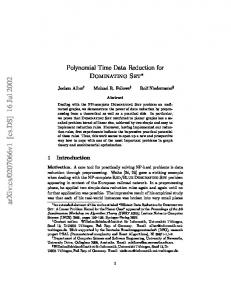
Fig. 1. The left-hand side shows the partitioning of the neighborhood of a single vertex v. The right-hand side shows the partitioning of a neighborhood N (v, w) of two vertices v and w. Since, in the left-hand figure, N3 (v) 6= ∅, reduction Rule 1 applies. In the right-hand figure, since N3 (v, w) cannot be dominated by a single vertex at all, Case 2 of Rule 2 applies √

approach presented in [4] immediately results in an O(c k · k + nO(1) ) Dominating Set algorithm on planar graphs (for some constant c). Also, the linear problem kernel directly proves the so-called “Layerwise Separation Property” [3] √ k for Dominating Set on planar graphs, again implying an O(c · k + nO(1) ) algorithm. Second, the linear problem kernel improves the time O(8k · n) search tree algorithm from [2] to an O(8k k + n3 ) algorithm. Apart from these theoretical results, we also underpin the practical importance of our approach through (ongoing) experimental studies. These indicate that the two proposed reduction rules can be implemented efficiently and lead to massive reductions on given input data. Notably, our data reductions also significantly accelerate implemented tree decomposition based algorithms for Dominating Set on planar graphs [6] due to an empirically observed reduction of the treewidth of the tested graphs. Due to the lack of space, many details had to be omitted and will appear in the full version of the paper.

2

The Reduction Rules

We present two reduction rules for Dominating Set. Both reduction rules are based on the same principle: We explore the local structure of the graph and try to replace it by a simpler structure. 2.1

The Neighborhood of a Single Vertex

Consider a vertex v ∈ V of the given graph G = (V, E). We partition the vertices of the neighborhood N (v) of v into three different sets N1 (v), N2 (v), and N3 (v) depending on what neighborhood structure these vertices have. More precisely, setting N [v] := N (v) ∪ {v}, we define N1 (v) := {u ∈ N (v) : N (u) \ N [v] 6= ∅}, N2 (v) := {u ∈ N (v) \ N1 (v) : N (u) ∩ N1 (v) 6= ∅}, N3 (v) := N (v) \ (N1 (v) ∪ N2 (v)).

LCNS, Vol 2368, pp. 150–159, Springer 2002

An example which illustrates the partitioning of N (v) into the subsets N1 (v), N2 (v), and N3 (v) can be seen in the left-hand diagram of Fig. 1. Based on the above definitions we give our first reduction rule. Rule 1 If N3 (v) 6= ∅ for some vertex v, then • remove N2 (v) and N3 (v) from G and • add a new vertex v ′ with the edge {v, v ′ }. Lemma 1. Let G = (V, E) be a graph and let G′ = (V ′ , E ′ ) be the resulting graph after having applied Rule 1 to G. Then γ(G) = γ(G′ ). Proof. Consider a vertex v ∈ V such that N3 (v) 6= ∅. The vertices in N3 (v) can only be dominated by either v or by vertices in N2 (v) ∪ N3 (v). But, clearly, N (w) ⊆ N (v) for every w ∈ N2 (v) ∪ N3 (v). This shows that an optimal way to dominate N3 (v) is given by taking v into the dominating set. This is simulated by the “gadget” {v, v ′ } in G′ . It is safe to remove N2 (v) ∪ N3 (v), since these vertices need not to be used in an optimal dominating set. Hence, γ(G′ ) = γ(G). ⊓ ⊔ Lemma 2. Rule 1 can be carried out in time O(n) for planar graphs and in time O(n3 ) for general graphs. 2 2.2

The Neighborhood of a Pair of Vertices

Similar to Rule 1, we explore the set N (v, w) := N (v) ∪ N (w) of two vertices v, w ∈ V . Analogously, we now partition N (v, w) into three disjoint subsets N1 (v, w), N2 (v, w), and N3 (v, w). Setting N [v, w] := N [v] ∪ N [w], we define N1 (v, w) := {u ∈ N (v, w) | N (u) \ N [v, w] 6= ∅}, N2 (v, w) := {u ∈ N (v, w) \ N1 (v, w) | N (u) ∩ N1 (v, w) 6= ∅}, N3 (v, w) := N (v, w) \ (N1 (v, w) ∪ N2 (v, w)). The right-hand diagram of Fig. 1 shows an example which illustrates the partitioning of N (v, w) into the subsets N1 (v, w), N2 (v, w), and N3 (v, w). Our second reduction rule—compared to Rule 1—is slightly more complicated. Rule 2 Consider v, w ∈ V (v 6= w) and suppose that N3 (v, w) 6= ∅. Suppose that N3 (v, w) cannot be dominated by a single vertex from N2 (v, w) ∪ N3 (v, w). Case 1 If N3 (v, w) can be dominated by a single vertex from {v, w}: (1.1) If N3 (v, w) ⊆ N (v) as well as N3 (v, w) ⊆ N (w): • remove N3 (v, w) and N2 (v, w) ∩ N (v) ∩ N (w) from G and • add two new vertices z, z ′ and edges {v, z}, {w, z}, {v, z ′ }, {w, z ′ }. (1.2) If N3 (v, w) ⊆ N (v), but not N3 (v, w) ⊆ N (w): • remove N3 (v, w) and N2 (v, w) ∩ N (v) from G and • add a new vertex v ′ and the edge {v, v ′ } to G. (1.3) If N3 (v, w) ⊆ N (w), but not N3 (v, w) ⊆ N (v): • remove N3 (v, w) and N2 (v, w) ∩ N (w) from G and

LCNS, Vol 2368, pp. 150–159, Springer 2002

• add a new vertex w′ and the edge {w, w′ } to G. Case 2 If N3 (v, w) cannot be dominated by a single vertex from {v, w}: • remove N3 (v, w) and N2 (v, w) from G and • add two new vertices v ′ , w′ and edges {v, v ′ }, {w, w′ }. Lemma 3. Let G = (V, E) be a graph and let G′ = (V ′ , E ′ ) be the resulting graph after having applied Rule 2 to G. Then γ(G) = γ(G′ ). Proof. Similar to the proof of Lemma 1, we observe that vertices from N3 (v, w) can only be dominated by vertices from M := {v, w} ∪ N2 (v, w) ∪ N3 (v, w). All cases in Rule 2 are based on the fact that N3 (v, w) needs to be dominated. All rules only apply if there is not a single vertex in N2 (v, w) ∪ N3 (v, w) which dominates N3 (v, w). We first of all discuss the correctness of Case (1.2) (and similarly the symmetric Case (1.3)): If v dominates N3 (v, w) (and w does not), then it is better to take v into the dominating set—and at the same time still leave the option of taking vertex w—than to take any combination of two vertices {x, y} from the set M \ {v}. It may be that we still have to take w to a minimum dominating set, but in any case {v, w} dominates at least as many vertices as {x, y}. The “gadget” {v, v ′ } simulates the effect of taking v. It is safe to remove N := (N2 (v, w) ∩ N (v)) ∪ N3 (v, w) since, by taking v into the dominating set, all vertices in N are already dominated and since, as discussed above, it is always better to take {v, w} into a minimum dominating set than to take v and any other of the vertices from N . In the situation of Case (1.1), we can dominate N3 (v, w) by both v or w. Since we cannot decide at this point which of these vertices should be chosen to be in the dominating set, we use the “gadget” with vertices v ′ and w′ which simulates a choice between v or w, as can be seen easily. In any case, however, it is better to take one of the vertices v and w (maybe both) than taking any two of the vertices from M \ {v, w}. The argument for this is similar to the one for Case (1.2). The removal of N3 (v, w) ∪ (N2 (v, w) ∩ N (v) ∩ N (w)) is safe by a similar argument than the one that justified the removal of N in Case (1.2). In Case 2, we need at least two vertices to dominate N3 (v, w). Since N (v, w) ⊇ N (x, y) for all pairs x, y ∈ M it is best to take v and w into the dominating set, simulated by the gadgets {v, v ′ } and {w, w′ }. As in the previous cases removing N3 (v, w) ∪ N2 (v, w) is safe since these vertices are already dominated and since these vertices need not be used for an optimal dominating set. 2 Lemma 4. Rule 2 can be carried out in time O(n2 ) for planar graphs and in time O(n4 ) for general graphs. 2 2.3

Reduced Graphs

Definition 1. Let G = (V, E) be a graph such that both the application of Rule 1 and the application of Rule 2 leave the graph unchanged. Then we say that G is reduced with respect to these rules.

LCNS, Vol 2368, pp. 150–159, Springer 2002

Observing that the (successful) application of any reduction rule always “shrinks” the given graph implies that there can only be O(n) successful applications of reduction rules. This leads to the following.3 Lemma 5. A graph G can be transformed into a reduced graph G′ with γ(G) = γ(G′ ) in time O(n3 ) in the planar case and in time O(n5 ) in the general case. 2

3

A Linear Problem Kernel for Planar Graphs

Here, we show that the reduction rules given in Section 2.1 yield a linear size problem kernel for dominating set on planar graphs. Theorem 1. For a planar graph G = (V, E) which is reduced with respect to Rules 1 and 2, we get |V | ≤ 335 γ(G), i.e., the dominating set problem on planar graphs admits a linear problem kernel. The rest of this section is devoted to sketch a proof of Theorem 1. The proof can be split into two parts. In a first step, we try to find a so-called “maximal region decomposition” of the vertices V of G. In a second step, we show, on the one hand, that such a maximal region decomposition must contain all but O(γ(G)) many vertices from V . On the other hand, we prove that such a region decomposition uses at most O(γ(G)) regions, each of which having size O(1). Combining the results then yields |V | = O(γ(G)). 3.1

Finding a Maximal Region Decomposition

Suppose that we have a reduced planar graph G with a minimum dominating set D. We know that, in particular, neither Rule 1 applies to a vertex v ∈ D, nor Rule 2 applies to a pair of vertices v, w ∈ D. We want to get our hands on the number of vertices that lie in neighborhoods N (v) for v ∈ D, or neighborhoods N (v, w) for v, w ∈ D. A first idea to prove that |V | = O(|D|) would be to find (at most O(|D|) many) neighborhoods N (v1 , w1 ), . . . , N (vℓ , wℓ ) with vi , wi ∈ D, such that all vertices in V lie in at least one such neighborhood; and then use the fact that G is reduced in order to prove that each N (vi , wi ) has size at most O(1). However, even if the graph G is reduced, the neighborhoods N (v, w) of two vertices v, w ∈ D may contain many vertices: the size of N (v, w) in a reduced graph basically depends on how big N1 (v, w) is. In order to circumvent these difficulties, we define the concept of a region R(v, w) for which we can guarantee that in a reduced graph it consists of only a constant number of vertices. Definition 2. Let G = (V, E) be a plane4 graph. A region R(v, w) between two vertices v, w is a closed subset of the plane with the following properties: 3

4

It must be emphasized here that our polynomial time bounds for the reduction rules give real worst-case bounds (which may not even be tight) and, in practice, the algorithms implementing these rules appear to be much faster. A plane graph is a particular planar embedding of a planar graph.

LCNS, Vol 2368, pp. 150–159, Springer 2002

00 11 0 1 00 11 0111111111111111111111 1 11111 00000 0 1 000 111 000000000000000000000 00 11 0 1 000 111 0000 1111 00000000000 11111111111 00000 11111 0111 1 000 000000000000000000000 0111111111111111111111 1 00000000000 11111111111 000 111 0000 1111 00000000000 11111111111 0 1 000 111 000000000000000000000 0111111111111111111111 1 00000000000 11111111111 000 111 0000 1111 00000000000 11111111111 0 1 000000000000000000000 111111111111111111111 00000000000 11111111111 000 111 00000000000 11111111111 000000000000000000000 111111111111111111111 00000000000 11111111111 0000000000000000 1111111111111111 0000 1111 00000000000000 11111111111111 00000000 11111111 000000000 111111111 00000000000 11111111111 000000000000000000000 111111111111111111111 00000000 11111111 0000000000000000 1111111111111111 00000000000000 11111111111111 000000000 111111111 0000 1111 00000000 11111111 000000000000000000000 111111111111111111111 00000000 11111111 0 1 0000000000000000 1111111111111111 0000 1111 00000000000000 11111111111111 00000000 11111111 000000000 111111111 000000000000000000000 111111111111111111111 00000000 11111111 000000 111111 0000 1111 0111111 1 0000000000000000 1111111111111111 0000 1111 00000000000000 11111111111111 00000000 11111111 000000000 00000000 11111111 000000 0000111111111 1111 000000000000000000000 111111111111111111111 0 1 0000000000000000 1111111111111111 0000 1111 00000000000000 11111111111111 00000000 11111111 000000000 111111111 00000000 11111111 000000 111111 000000000000000000000 111111111111111111111 0000 1111 0 1 0000000000000000 1111111111111111 0000 1111 00000000000000 11111111111111 00000000 11111111 000000000 111111111 00000000 11111111 00 11 000000000000000000000 111111111111111111111 0000 1111 0000000000000000 1111111111111111 00000000000000 11111111111111 000000000 111111111 0000 1111 00000000 11111111 00000000 11111111 00 11 000000000000000000000 111111111111111111111 0000 1111 0000000000000000 1111111111111111 0000 1111 00000000000000 11111111111111 00000000 11111111 000000000 111111111 00000000 11111111 00000000 11111111 000000000000000000000 111111111111111111111 0000 1111 0000000000000000 1111111111111111 0000 1111 00000000000000 11111111111111 00000000 11111111 000000000 00000000 11111111 00000000 11111111 0000111111111 1111 000000000000000000000 111111111111111111111 0000000000000000 1111111111111111 0000 1111 00000000000000 11111111111111 00000000 11111111 000000000 111111111 11111111111111111 00000000000000000 000000000000 111111111111 00000000000000000 11111111111111111 000000 111111 111 000 00000 11111 00000000 11111111 00000000 11111111 000000000000000000000 111111111111111111111 00000 11111 0000000000000000 1111111111111111 0000 1111 00000000000000 11111111111111 000000000 111111111 000000000000 111111111111 00000000000000000 11111111111111111 000000 111111 00000 11111 00000 11111 0000000000000000 1111111111111111 0000 1111 000000000000000 111111111111111 000000000000 111111111111 00000000000000000 11111111111111111 000000 111111 00000 11111 0000000000000000 1111111111111111 0000 1111 000000000000000 111111111111111 000000000000 111111111111 00000000000000000 11111111111111111 000000 111111 0000000000000000 1111111111111111 Fig. 2. The left-hand side diagram shows an example of a possible D-region decomposition R of some graph G, where D is the subset of vertices in G that are drawn in black. The various regions are highlightened by different patterns. The remaining white areas are not considered as regions. Note that the given D-region decomposition is maximal. The right-hand side shows the induced graph GR (Definition 4)

1. the boundary of R(v, w) is formed by two paths P1 and P2 in V which connect v and w, and the length of each path is at most three5 , and 2. all vertices which are strictly inside6 the region R(v, w) are from N (v, w). For a region R, let V (R) denote the vertices belonging to R, i.e., V (R) := {u ∈ V | u sits inside or on the boundary of R}. Definition 3. Let G = (V, E) be a plane graph and D ⊆ V . A D-region decomposition of G is a set R of regions between pairs of vertices in D, such that 1. for R(v, w) ∈ R no vertex from D (except for v, w) lies in V (R(v, w)), and 2. no two regions R1 , R2 ∈ R do intersect (however, they may touch each other by having common boundaries). S For a D-region decomposition R, we define V (R) := R∈R V (R). A D-region decomposition R is called maximal if there is no region R ∈ / R such that R′ := ′ R ∪ {R} is a D-region decomposition with V (R) ( V (R ). For an example of a (maximal) D-region decomposition we refer to the left-hand side diagram of Fig. 2. It is not directly clear, whether, for a given graph G with dominating set D, a maximal D-region decomposition of G exists. We will see that this indeed is the case. Moreover, we will show that we can even find a special maximal D-region decomposition. For that purpose, we observe that a D-region decomposition induces a graph in a very natural way. Definition 4. The induced graph GR = (VR , ER ) of a D-region decomposition R of G is the graph with possible multiple edges which is defined as follows: VR := D, and ER := {{v, w} | there is a region R(v, w) ∈ R between v, w ∈ D}. 5 6

The length of a path is the number of edges on it. i.e., not sitting on the boundary of R(v, w)

LCNS, Vol 2368, pp. 150–159, Springer 2002

Worst-case scenario for a region R(v, w): u2 u1

v

1111111111111111 0000000000000000 0000 1111 00000 11111 0000 1111 00000 11111 0000000000000000 1111111111111111 0000 1111 00000 11111 0000 1111 00000 11111 0000000000000000 1111111111111111 0000 1111 00000 11111 0000 1111 0 1 00000 11111 0000000000000000 1111111111111111 0000 1111 0 1 00000 11111 0000 1111 0 1 00000 11111 0000000000000000 1111111111111111 0000 1111 0 1 00000 11111 0000 1111 0 1 00000 11111 0000000000000000 1111111111111111 0000 0 1 01111 1 00000 11111 0000 0 1 01111 1 00000 11111 0000000000000000 1111111111111111 0000 1111 0 1 d 0 1 000001 11111 0000 w 1111 0000000000 1111111111 0000000000 1111111111 0 0 1 00000 11111 0000000000000000 1111111111111111 0000 1111 0 1 00000 11111 0000 1111 0000000000 1111111111 0000000000 1111111111 0000000000000000 1111111111111111 00000 11111 0000000000000000 1111111111111111 0000 1111 00000 11111 0000 1111 0000000000 1111111111 0000000000 1111111111 0000000000000000 1111111111111111 00000 11111 0000 1111 00000 11111 0000 1111 0000000000000000 1111111111111111 00000 11111 0000 1111 00000 11111 0000 1111 0000000000000000 1111111111111111 00000 11111 0000 1111 00000 11111 0000 1111 0000000000000000 1111111111111111 00000 11111 0000 1111 00000 11111 0000 1111 0000000000000000 1111111111111111 00000 11111 0000 1111 00000 11111 0000 1111 0000000000000000 1111111111111111 00000 11111 0000 1111 00000 11111 0000 1111 0000000000000000 1111111111111111 00000 11111 0000 1111 00000 11111 0000 1111 0000000000000000 1111111111111111 00000 11111 u3

u4

Simple regions S(x, y):

0 01 1 0 1 11111111111111 00000000000000 0 1 0x 1 00000000000000 11111111111111 0 1 Type 2: 00000000000000 11111111111111 00000000000000 11111111111111 00 0000000000000011 11111111111111 00 11 00000000000000 11111111111111 00000000000000 11111111111111 0 1 01 1 00000000000000 11111111111111 0y 111111111 0 1 000000000 0 1 00000000000000 11111111111111 0 1 0 1 000000000 111111111 01 1 0x 000000000 0 111111111 01 1 000000000 111111111 000000000 111111111 0 1 000000000 111111111 000000000 0 1 Type 1: 111111111 000000000 111111111 11111 00000 111 000 000 111 00 11 0 1 000000000 111111111 000000000 111111111 00 11 000 111 000000000 111111111 0 1 000000000 111111111 000 111 000000000 111111111 0 1 000000000 111111111 000 111 000000000 111111111 0 1 000000000 111111111 000 111 0 1 0y 01 1 0 1

Fig. 3. The left-hand diagram shows a worst-case scenario for a region R(v, w) between two vertices v and w in a reduced planar graph (cf. the proof of Proposition 3). Such a region may contain up to four vertices from N1 (v, w), namely u1 , u2 , u3 , and u4 . The vertices from R(v, w) which belong to the sets N2 (v, w) and N3 (v, w) can be grouped into so-called simple regions of Type 1 (marked with a line-pattern) or of Type 2 (marked with a crossing-pattern); the structure of such simple regions S(x, y) is given in the right-hand part of the diagram. In R(v, w) there might be two simple regions S(d, v) and S(d, w) (of Type 2), containing vertices from N3 (v, w). And, we can have up to six simple regions of vertices from N2 (v, w): S(u1 , v), S(v, u3 ), S(u4 , w), S(w, u2 ), S(u2 , v), and S(u4 , v) (among these, the latter two can be of Type 2 and the others are of Type 1)

Note that, by Definition 3, the induced graph GR of a D-region decomposition is planar. For an example of an induced graph GR see Fig. 2. Definition 5. We say that a planar graph G = (V, E) with multiple edges is thin, if there exists a planar embedding such that the following property holds: If there are two edges e1 , e2 between a pair of distinct vertices v, w ∈ V , then there must be two further vertices u1 , u2 ∈ V which sit inside the two disjoint regions of the plane that are enclosed by e1 , e2 . Lemma 6. For a thin planar graph G = (V, E) we have |E| ≤ 3|V | − 6. Proof. The claim is true for planar graphs without multiple edges. An easy induction on the number of multiple edges in G proves the claim. ⊓ ⊔ Using the notion of thin graphs, we can formulate the main result of this section. Proposition 1. For a reduced plane graph G with dominating set D, there exists a maximal D-region decomposition R such that GR is thin. 2 3.2

Region Decompositions and the Size of Reduced Planar Graphs

Suppose that we are given a reduced planar graph G = (V, E) with a minimum dominating set D. Then, by Proposition 1 and Lemma 6, we can find a maximal

LCNS, Vol 2368, pp. 150–159, Springer 2002

D-region decomposition R of G with at most O(γ(G)) regions. In order to see that |V | = O(γ(G)), it remains to show that (1) there are at most O(γ(G)) vertices which do not belong to any of the regions in R, and that (2) every region of R contains at most O(1) vertices. These issues are treated by the following two propositions, the extensive proofs of which are omitted. Proposition 2. Let G = (V, E) be a plane reduced graph and let D be a dominating set of G. If R is a maximal D-region decomposition, then R contains all but O(|D| + |R|) vertices of G. More precisely, |V \ V (R)| ≤ 2|D| + 56|R|. 2 We now investigate the maximal size of a region in a reduced graph. The worstcase scenario for a region in a reduced graph is depicted in Fig. 3. Proposition 3. A region R of a plane reduced graph contains at most 55 vertices, i.e., |V (R)| ≤ 55. 2 To prove Theorem 1 we first of all observe that, for a graph G with minimum dominating set D, by Proposition 1 and Lemma 6, we can find a D-region decomposition R of G with at mostP 3γ(G) regions, i.e., |R| ≤ 3γ(G). By Proposition 3, we know that |V (R)| ≤ R∈R |V (R)| ≤ 55|R|. By Proposition 2, we have |V \ V (R)| ≤ 2|D| + 56|R|. Hence, we get |V | ≤ 2|D| + 111|R| ≤ 335 γ(G).

4

Conclusion

Presenting two simple and easy to implement reduction rules for Dominating Set, we proved that for planar graphs a linear size problem kernel can be efficiently constructed. Our result complements and partially improves previous results [1–4] on the parameterized complexity of Dominating Set on planar graphs. We emphasize that the proven bound on the problem kernel size is a pure worst-case upper bound. In first experimental studies to be reported elsewhere, we obtained much smaller problem kernels. An immediate open question is whether or not we can improve the constant factor to values around 10. This would bring the problem kernel for Dominating Set on planar graphs into “dimensions” as known for Vertex Cover, where it is of size 2k [8]. This could be done by either improving the analysis given or (more importantly) further improving the given reduction rules or both. Improving the rules should be doable by further extending the concept of neighborhood to more than two vertices. From a practical point of view, however, one also has to take into account to keep the reduction rules as simple as possible in order to avoid inefficiency due to increased overhead. It might well be the case that additional, more complicated reduction rules only improve the worst case bounds, but are of little or no practical use due to their computational overhead. Acknowledgements. For two years, besides ourselves the linear size problem kernel question for Dominating Set on planar graphs has taken the attention of numerous people, all of whom we owe sincere thanks for their insightful and inspiring remarks and ideas. Among these people we particularly would like to mention Frederic Dorn, Henning Fernau, Jens Gramm, Michael Kaufmann, Ton Kloks, Klaus Reinhardt, Fran

LCNS, Vol 2368, pp. 150–159, Springer 2002

Rosamond, Peter Rossmanith, Ulrike Stege, and Pascal Tesson. Special thanks go to Henning for the many hours he spent with us on “diamond discussions” and for pointing us to a small error concerning the application of the linear problem kernel, and to Frederic for again doing a perfect implementation job, which also uncovered a small error in a previous version of Rule 2.

References 1. J. Alber, H. L. Bodlaender, H. Fernau, and R. Niedermeier. Fixed parameter algorithms for planar dominating set and related problems. In Proc. 7th SWAT 2000 , Springer-Verlag LNCS 1851, pp. 97–110, 2000. 2. J. Alber, H. Fan, M. R. Fellows, H. Fernau, R. Niedermeier, F. Rosamond, and U. Stege. Refined search tree technique for dominating set on planar graphs. In Proc. 26th MFCS 2001 , Springer-Verlag LNCS 2136, pp. 111-122, 2001. 3. J. Alber, H. Fernau, and R. Niedermeier. Parameterized complexity: exponential speed-up for planar graph problems. In Proc. 28th ICALP 2001 , Springer-Verlag LNCS 2076, pp. 261–272, 2001. 4. J. Alber, H. Fernau, and R. Niedermeier. Graph separators: a parameterized view. In Proc. 7th COCOON 2001 , Springer-Verlag LNCS 2108, pp. 318–327, 2001. 5. J. Alber, J. Gramm, and R. Niedermeier. Faster exact solutions for hard problems: a parameterized point of view. Discrete Mathematics, 229: 3–27, 2001. 6. J. Alber and R. Niedermeier. Improved tree decomposition based algorithms for domination-like problems. In Proc. 5th LATIN 2002 , Springer-Verlag LNCS 2286, pp. 613-627, 2002. 7. R. Bar-Yehuda and S. Even. A local-ratio theorem for approximating the weighted vertex cover problem. Annals of Discrete Mathematics, 25: 27–46, 1985. 8. J. Chen, I. A. Kanj, and W. Jia. Vertex cover: further observations and further improvements. Journal of Algorithms, 41:280–301, 2001. 9. R. G. Downey and M. R. Fellows. Parameterized computational feasibility. In P. Clote, J. Remmel (eds.): Feasible Mathematics II, pp. 219–244. Birkh¨ auser, 1995. 10. R. G. Downey and M. R. Fellows. Parameterized Complexity. Monographs in Computer Science. Springer-Verlag, 1999. 11. M. R. Fellows. Parameterized complexity: the main ideas and some research frontiers. In Proc. 12th ISAAC 2001, Springer-Verlag LNCS 2223, pp. 291–307, 2001. 12. T. W. Haynes, S. T. Hedetniemi, and P. J. Slater. Fundamentals of Domination in Graphs. Monographs and textbooks in pure and applied Mathematics Vol. 208, Marcel Dekker, 1998. 13. G. L. Nemhauser and L. E. Trotter. Vertex packing: structural properties and algorithms. Mathematical Programming, 8:232–248, 1975. 14. F. S. Roberts. Graph Theory and Its Applications to Problems of Society. SIAM Press 1978. Third printing 1993 by Odyssey Press. 15. J. A. Telle. Complexity of domination-type problems in graphs. Nordic J. Comput. 1:157–171, 1994. 16. K. Weihe. Covering trains by stations or the power of data reduction. In Proc. 1st ALEX’98 , pp. 1–8, 1998. 17. K. Weihe. On the differences between “practical” and “applied” (invited paper). In Proc. WAE 2000 , Springer-Verlag LNCS 1982, pp. 1–10, 2001.