Previous work on efficient customized processor design primarily focused on in-order architectures. However, with the recent introduction of out-of-order ...
Efficient Design Space Exploration of High Performance Embedded Out-of-Order Processors Stijn Eyerman Lieven Eeckhout Koen De Bosschere ELIS, Ghent University, Sint-Pietersnieuwstraat 41, B-9000 Gent, Belgium {seyerman,leeckhou,kdb}@elis.UGent.be Abstract Previous work on efficient customized processor design primarily focused on in-order architectures. However, with the recent introduction of out-of-order processors for highend high-performance embedded applications, researchers and designers need to address how to automate the design process of customized out-of-order processors. Because of the parallel execution of independent instructions in outof-order processors, in-order processor design methodologies which subdivide the search space in independent components are unlikely to be effective in terms of accuracy for designing out-of-order processors. In this paper we propose and evaluate various automated single- and multi-objective optimizations for exploring out-of-order processor designs. We conclude that the newly proposed genetic local search algorithm outperforms all other search algorithms in terms of accuracy. In addition, we propose two-phase simulation in which the first phase explores the design space through statistical simulation; a region of interest is then simulated through detailed simulation in the second phase. We show that simulation time speedups can be obtained of a factor 2.2X to 7.3X using two-phase simulation.
1. Introduction High performance embedded applications such as multimedia, networking, imaging, high end consumer applications, etc. are an important market segment today. And because of the high performance requirements of these embedded applications, computer companies move into (or did already move into) using out-of-order processors. Examples are NEC’s VR55000 and VR77100 Star Sapphire and SandCraft’s SR710X0 64-bit MIPS processors. For these high end embedded systems it is extremely important to optimize the design for a given application or a given set of applications with a limited engineering effort. The design question then is how to organize the microprocessor’s microarchitecture, i.e., how big should the caches be, what should the processor width be, how many in-flight instructions should there be, etc. A lot of prior work has been done on automated design space exploration methodologies for in-order (incl. VLIW) architectures, see for example PICO [8], Sherpa [13] and the
references therein. The in-order processor design methodologies often assume that the whole system can be broken up into independent subcomponents. Each of those subcomponents then gets optimized before reassembling the whole system. Because of the complex interactions in out-of-order processors such as parallel executions of independent instructions, latency hiding mechanisms, speculative execution, etc., it is unlikely that these design methodologies can be used for customized out-of-order processor design. In this paper we propose the use of automated design space exploration for efficiently exploring the out-of-order processor design space. We evaluate various single-objective and multi-objective search algorithms and propose genetic local search as a new single-objective search algorithm that outperforms all other search algorithms in terms of accuracy. In addition, we also propose two-phase simulation to prune the design space. The idea is to explore the design space quickly using a fast simulation technique as a first step. And we propose statistical simulation for this purpose. We then explore a small region of interest identified in the first phase through detailed (and thus slower) cycle-accurate architectural simulation. The overall simulation speedup obtained through two-phase simulation is 2.2X to 7.3X in our experiments. And we show that two-phase simulation can be applied to single-objective as well as to multi-objective optimization criteria.
2. Previous work There exists a lot of work on design space exploration. Obviously, we cannot discuss the whole literature written on this topic. For a detailed description on design space exploration techniques, we refer to [5]. Since our main contributions are on design space pruning and automated design space exploration, we will revisit some of those.
2.1. Design space pruning A first approach to reducing the total simulation time is to prune the design space through what could be called hierarchical design space exploration. Hekstra et al. [6] for example describe how they explored the TriMedia CPU64 design. In order to explore the huge design space, they first probe the design space in order to identify the architectural parameters that affect overall performance the most. These
corner cases then determine bounds on specific design parameters which reduces the design space to be explored in detail. Mohanty et al. [9] first uses constraint analysis to prune the design space of a heterogeous system design. The pruned design space is then explored using a set of component-specific high-level simulation models and system-wide performance estimation. In a final step, the complete system is simulated in a low-level cycle-accurate simulation model. The two-phase simulation approach that we propose in this paper is orthogonal to the hierarchical design space exploration methodology proposed by Mohanty et al. Indeed, the two-phase simulation can be used for example in the second and third step of Mohanty et al.’s methodology as a replacement for the architectural cycle-accurate simulations. This could yield significant simulation time reductions.
2.2. Automated design space exploration In this paper we evaluate a number of design space exploration techniques that were previously proposed in the context of electronic design, such as random descent, steepest descent (hill climbing) [14], one-parameterat-a-time [4], genetic search for single-objective optimizations [15] and multi-objective optimizations [12] and tabu search [1]. In this paper we also evaluate genetic local search which is, to the best of our knowledge, not previously evaluated within the context of electronic design. Jaszkiewicz [7] proposed genetic local search as a single-objective search algorithm. The basic idea is to do a locally optimized search of each design point in a generation before recombination occurs during a genetic/evolutionary search. Our results show that genetic local search outperforms all the other search algorithms in terms of accuracy.
3. Design space exploration We explore both single- and multi-objective optimizations in this paper for exploring out-of-order microarchitectures.
3.1. Single-objective optimization We first discuss the six single-objective optimization algorithms that we evaluate in this paper. Random descent (RD) randomly picks a dimension at each iteration of the search algorithm and randomly increases or decreases the microarchitectural parameter along that dimension. If the objective function improves, the new design point is accepted; otherwise, another dimension is chosen. The algorithm terminates whenever the objective function no longer improves. Steepest descent (SD), also refered to as hill climbing, does not randomly select a dimension along which to optimize, but chooses the dimension along which the objective function improves the most. This is done by examining all the neighboring design points. The dimension along which the steepest slope is observed is then selected. The advantage of steepest descent over random descent is that there
are fewer iterations in the search algorithm, however, per iteration there is more work to be done, i.e., all the neighboring design points need to be evaluated whereas random descent randomly picks a dimension. One parameter at a time (OP) follows a fixed ordering of dimensions along which to optimize. When optimizing a dimension, all possible values along that dimension are evaluated and the optimal design point is then retained. And this is done for all dimensions in a fixed ordering. When this ordering is completely scanned, we start over again until the objective function no longer improves. The ordering that we use is the sensitivity-based ordering proposed by Fornaciari et al. [4]. Tabu search (TS) resembles steepest descent, i.e., it examines all neighboring design points and goes in the direction with the optimal objection function. The important difference with steepest descent however is that tabu search always goes in that direction, irrespective of whether the objective function in that design point is better than in the current design point. This is to avoid local minima. Tabu search also keeps track of a tabu list which contains a number of previously taken directions. In order not to circulate around local minima, tabu search never goes in a direction that appears in the tabu list. There is however one exception, tabu search can accept a direction that results in a design point with a better objective function than all previously visited design points. Genetic search (GS) starts from a randomly chosen generation of design points. It then randomly walks those points until all constraints are met—the objective function is not optimized. From those design points, a new generation is built. This is done by selecting the best performing design points found so far, complemented with a number of other design points probabilistically chosen from the remaining design points using weights that are correlated to their respective objective function values. On these selected design points, mutation and crossover is applied which yields us a new generation. From there on, the search algorithm is iterated. Genetic local search (GLS) is an optimized version of the genetic search algorithm. The key difference is that for each generation, genetic local search fully optimizes each design point in a generation using a random descent algorithm, i.e., the objective function is optimized while meeting the constraints for each design point in the generation. GLS can thus be viewed of as a genetic algorithm applied on locally optimized solutions.
3.2. Multi-objective optimization In contrast to single-objective optimizations, multiobjective optimizations strive at identifying a set of so called pareto-optimal design points according to a number of objective functions. A pareto-optimal design point is a design point for which there exist no other points in the design space that achieve a better score for all objective functions. Once the set of pareto-optimal design points is identified from a multi-objective design space exploration, the system designer can then select a design point that trades off the various objective functions.
The multi-objective search algorithm that we use in this paper is called SPEA2 [17] which is an improved version of the well-established Strength Pareto Evolutionary Algorithm (SPEA) [18]. This algorithm is an elitist evolutionary algorithm that keeps track of the best solutions found so far. Potentially new pareto-optimal design points are created through recombination and mutation much like what is being done in the genetic search algorithms mentioned previously. The algorithm finalizes when a fixed number of iterations have been performed. The end result of the SPEA2 algorithm is a set of pareto-optimal design points. For a more in-depth discussion on SPEA2, we refer to [17, 18].
4. Two-phase simulation The motivation for going into two-phase simulation is that detailed cycle-by-cycle simulations are infeasible, if not impossible, for exploring huge design spaces. Since the simulation of one single design point may take multiple hours, exploring a large design space exhaustively is impossible. Even when using an efficient search algorithm, the number of design points to be explored rapidly becomes fairly large which makes detailed simulation throughout the design space exploration infeasible. The idea behind two-phase simulation is as follows. During a first phase of the design space exploration, we employ a fast simulation technique to quickly explore the design space. Compared to detailed simulation, the fast simulation technique should be several orders of magnitude faster, yet achieve good relative accuracy. The end result of the first phase then is a region of interest that achieves near-optimal performance. This region of interest then is to be explored through more detailed (and slower) cycle-by-cycle simulations. Because of the fact that this region is much smaller than the original space, the overall simulation time is reduced substantially. For the single-objective optimizations, two-phase simulation works as follows. We first use a fast simulation technique to explore the design space using a design space exploration algorithm. Once this search algorithm is terminated, we then go into the second phase and explore through detailed simulation a small region around the optimum found in the first phase. This small region is defined as the region where the fast simulation technique observes a deviation that is smaller than x% from the optimum’s objective function value. In order to clarify what the value of x% should be, we first discuss the relation between absolute and relative error rates. Absolute error for a metric M in a design point A is defined as: AE =
MF,A − MD,A , MD,A
with F and D standing for fast and detailed simulation, respectively. The absolute error quantifies the prediction in a single design point. Relative error between two design points A and B on the other hand, is defined as: RE = MF,B /MF,A − MD,B /MD,A .
The relative error thus quantifies the error when predicting the performance increase or decrease between multiple design points. As mentioned above, the search space during the second phase of the design space exploration is limited by the relative error threshold x%. The exact value to be assigned to x depends on the relative accuracy of the fast simulation technique that is being used. It’s important to note here that this threshold can be set fairly tight because the relative accuracy of a fast simulation technique is usually better than its absolute accuracy. This will limit the search space during detailed simulation substantially. The assumption being made here by setting the relative error threshold x% is that a relative increase (or decrease) larger than x% identified by the fast simulation technique is unlikely to correspond to a decrease (or increase) when measured through detailed simulation. For the fast simulation technique that we use in this paper, namely statistical simulation, we use a 3% relative error threshold. Obviously, choosing an appropriate relative error threshold depends on the quality of the fast simulation technique. The higher the relative accuracy of a given fast simulation technique, the lower the threshold can be set, and thus the smaller the overall simulation time during design space exploration. For the multi-objective optimizations, two-phase simulation works similarly. The fast simulation technique explores the design space in the first phase using for example SPEA2. This yields a set of pareto-optimal design points according to the fast simulation technique. The second phase which uses detailed simulation then starts from those design points. Since the fast simulation technique explored most of the design space already, the number of iterations can now be lowered in the second phase. This results in substantial overall simulation time reductions.
5. Statistical simulation The fast simulation technique that is used in the first phase in two-phase simulation can be any fast simulation technique of interest. In this paper, we propose the use of statistical simulation which was previously shown to be highly accurate for modeling out-of-order processors [3, 10, 11]. Absolute error rates are reported of 6% on average. The relative error rate is lower, typically less than 3%. Other alternatives such as analytical models or sampling are less appropriate for this application; accurate analytical modeling is difficult to obtain for out-of-order processors, and sampling requires more simulated instructions than what is required for statistical simulation which would limit the benefits of two-phase simulation. Statistical simulation works in three steps. First, a program execution is profiled by measuring a number of program characteristics. In statistical profiling we make a distinction between microarchitecture-independent and microarchitecture-dependent characteristics. The microarchitecture-independent characteristics are metrics such as instruction mix, control flow transition probabilities between basic blocks and inter-operation dependency distributions. The microarchitecture-dependent characteristics are metrics related to locality events, such as cache miss rates and branch mispredict rates. The reason for mea-
description audio decoding image decompression image decompression image compression 3-D graphics speech recognition
input S 16 44 titanic3 monalisa monalisa tst ex5 c1.wav
insn cnt (M) 11.1 11.7 41.4 149.2 128.0 24.9
Table 1. The MediaBench benchmarks used in this study along with their inputs and dynamic instruction count (in millions).
suring these statistics in a microarchitecture-dependent way is that they are hard to predict in a microarchitectureindependent way. This does not affect the applicability of this methodology for efficient design space exploration. Techniques exist for measuring these locality metrics efficiently by simulating multiple configurations in parallel in a single profiling run [16]. Note that profiling the application needs to be done only once throughout the complete design space exploration. In the second step, a synthetic trace is then produced from this statistical profile. The synthetic trace then resembles the original program trace in a statistical sense. The important benefit however is that the synthetic trace is extremely short in comparison to the original trace; the synthetic traces that we use in this paper for example only contain 500K instructions. In the third and final step, this synthetic trace is then simulated on a statistical trace-driven simulator. This statistical simulator is very simple in nature since it does not model branch predictors nor caches—these structures are modeled statistically. For example, when a mispredicted branch gets executed, the pipeline is flushed and new instructions are fetched as if they come from the correct control flow path. For a D-cache miss, the latency for the next level in the memory hierarchy is assigned. An I-cache miss stops the fetching of new instructions into the pipeline for a number of cycles.
6. Experimental setup 6.1. Simulation infrastructure We use the sim-outorder simulator from the SimpleScalar Tool Set v3.01 which is a detailed cycle-by-cycle superscalar processor simulator. This simulator is augmented with Wattch v.012 for obtaining energy consumption numbers from architectural simulation runs. The benchmarks used in this paper are taken from the MediaBench suite3 , see Table 1.
6.2. Design space The design space that we explore is huge. We vary 15 microarchitectural parameters in total; and each of them can be varied over 2 to 5 parameter values. The parameters that we 1 2 3
http://www.simplescalar.com http://www.eecs.harvard.edu/∼dbrooks/ http://www.icsl.ucla.edu/∼billms/
1600 1400
number of simulations
benchmark rawdaudio unepic djpeg cjpeg texgen rasta
1200
RD
1000
OP SD
800
TS
600
GS
400
GLS
200 0 rawdaudio
unepic
rasta
texgen
cjpeg
djpeg
avg
Figure 1. The number of simulations during design space exploration for single-objective optimization.
vary are the processor width (2-issue up to 10-issue), the instruction window size (32-entry up to 128-entry), the number of functional units for each type (1 up to 8), the branch predictor size (512 entries up to 4K entries), the cache sizes (8KB up to 128KB for L1 caches; 256KB up to 4MB for L2), etc. In total, the design space contains 1.6 billion possible design points to be explored. Obviously, we did not explore this huge design space through an exhaustive search. By consequence, the optimal design point for the singleobjective optimization is also unknown. To get around this, the optimal design point ever found by all of our search algorithms is considered as our reference point. All errors reported are relative to this reference point. This does not affect the general conclusions from this paper however; the errors are still useful for comparing the various search algorithms.
6.3. Objective functions For the single-objective optimization runs, we consider the following objective function. We optimize the design for minimal energy while guaranteeing a target level of performance, i.e., for a given level of performance, we minimize the energy consumption. For the multi-objective optimizations, we explore the design space by trading energy consumption versus performance, i.e., we explore the paretooptimal design points as a function of performance and energy.
7. Evaluation We now evaluate the automated design space exploration techniques that we propose in this paper. Subsequently, we will evaluate the simulation time speedups that are obtained from two-phase simulation.
7.1. Automated design space exploration Figures 1 shows the number of simulations that each of the single-objective search algorithms require. We observe that random descent and one-parameter-at-a-time are fast search algorithms, i.e., the number of simulation is very limited (163 and 139 on average for RD and OP, respectively). The other search algorithms require significantly more simulations before the search algorithm finds a stable solution.
25%
RD OP
15%
SD TS
10%
GS GLS
5% 0% rawdaudio
unepic
rasta
texgen
cjpeg
djpeg
avg
Figure 2. The percentual deficiency of the optima found by the various search algorithms.
energy per instruction (EPI)
20%
% deficiency
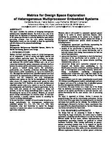
detailed simulation (50 iters)
6.5
detailed simulation (20 iters)
6
two-phase simulation (5 iters)
5.5 5 4.5 4 3.5 0.3
0.4
0.5
0.6
0.7
cycles per instruction (CPI)
3.0%
TS/RD TS/OP
2.5%
% deficiency
Figure 4. The pareto-optimal design points found through detailed and two-phase simulation for unepic.
TS/SD TS/TS
2.0%
OP/RD OP/OP
1.5%
OP/SD OP/TS
1.0%
SD/RD SD/OP
0.5%
SD/SD SD/TS
0.0% 0
200
400 number of simulations
600
800
GS/GS GLS/GLS
Figure 3. Deficiency is plotted against total simulation time for the various two-phase simulation approaches.
SD requires 617 simulations on average; TS, GS and GLS require 892, 993 and 1004 simulations, respectively. Figure 2 shows the accuracy of the various search algorithms. The deficiencies reported in this graph are the relative deviation in energy consumption for the optima found by the various search algorithms compared to the global optimum. (Recall that we refer to the global optimum as the best solution found by all search algorithms.) We observe that random descent, one-parameter-at-a-time, steepest descent and tabu search can result in solutions that are significantly worse (up to 23% off) than the solutions found by genetic search and genetic local search. We thus conclude that genetic search and genetic local search are the most accurate search algorithms; they seem to be able to avoid local optima more efficiently. However, as mentioned above, this comes at the cost of a relatively larger number of simulations that need to be run during the search algorithm.
7.2. Two-phase simulation The results shown so far assumed detailed simulation throughout the entire design space exploration. We now quantify the simulation time speedup when two-phase simulation is used instead of detailed simulation.
Single-objective optimization. We first evaluate the benefit of two-phase simulation for single-objective optimization. Figure 3 shows the various two-phase search algorithms as a function of deficiency on the Y axis versus simulation time on the X axis. These numbers are average numbers over all the benchmarks. Obviously, the closer to the origin, the better. The simulation time plotted here is measured in units of full length simulations; we include the simulation time required for the statistical simulation runs into the total simulation time. We considered various combinations of search algorithms to be used in the first phase and the second phase in order to explore the possibilities and the interactions between the first and second phase. Note that for the genetic algorithms (GS and GLS), we cannot combine them with the other approaches because a generation is required at each step in the search algorithm which is not provided by the non-genetic algorithms. We observe that under two-phase simulation, genetic local search remains the most accurate search algorithm. Comparing GLS under detailed simulation (Figure 1) vs. GLS under two-phase simulation (GLS/GLS in Figure 3), we conclude that two-phase simulation improves the overall simulation speed by a factor 2.2X. In addition, the deficiency under two-phase simulation is similar to the deficiency under detailed simulation. Another search algorithm that performs very well in terms of accuracy versus simulation time is steepest descent. Comparing SD under detailed simulation vs. SD/SD we observe a simulation speedup of a factor 7.3X for the same accuracy. The reason why steepest descent benefits more from two-phase simulation than the other search algorithms is that steepest descent optimizes the objective function through a local search whereas the other algorithms perform a broader search. Once steepest descent gets close to the optimum, it finds the optimum very quickly. Multi-objective optimization. Two-phase simulation can also be used for multi-objective optimization. Figure 4 shows the pareto-optimal design points
benchmark unepic djpeg texgen rasta
HVR (20 iters) 0.910 0.876 0.943 0.895
HVR (2-phase/5 iters) 0.985 0.909 0.944 0.902
Table 2. HVR values compared to 50 detailed simulation iterations for multi-objective optimization using (i) 20 detailed simulation iterations and (ii) two-phase simulation with only 5 detailed simulation iterations.
(EPI vs. CPI) for the unepic benchmark and the following three scenarios. In the first scenario we use 50 iterations using detailed simulation. The second scenario uses 20 iterations under detailed simulation. The third scenario uses two-phase simulations in which there are only 5 iterations done under detailed simulation. We observe that two-phase simulation allows for finding similar pareto-optimal design points as through detailed simulation. Note that two-phase simulation yields a better pareto curve than 20 detailed simulations scenario. This graph implies that two-phase simulation achieves approximately the same accuracy as the 50 iterations using detailed simulation while requiring 10 times less detailed simulations—the statistical simulation runs are done very quickly and account for a very small fraction of the total simulation time. We also compare these pareto curves more rigorously using the hypervolume ratio (HVR) metric discussed in [2]. The hypervolume metric takes into account closeness and diversity of the pareto curves compared to a reference pareto curve; our reference curve is the 50 detailed simulation iterations. Table 2 shows the HVR metrics for the various benchmarks under two-phase simulation. The closer the HVR values are to one, the better. We clearly observe that high HVR values are obtained for two-phase simulation and they are higher than the 20 iterations under detailed simulation. We thus conclude that two-phase simulation can yield substantial simulation time speedups with only a very small loss in accuracy.
8. Conclusion This paper discussed design space exploration techniques for the efficient and automated design of out-of-order microarchitectures for high performance embedded processors. We proposed and evaluated various search algorithms for exploring the microarchitectural design space and concluded that the newly proposed genetic local search algorithm outperforms the other algorithms in terms of accuracy. In addition, we presented two-phase simulation which explores the design space first using statistical simulation in order to identify a small region of interest. This region is then further explored through detailed simulation. This yields substantial simulation time speedups in the order of 2.2X to 7.3X. We showed that two-phase simulation is applicable to both single- and multi-objective optimizations.
Acknowledgements Stijn Eyerman and Lieven Eeckhout are supported by the Fund for Scientific Research—Flanders (Belgium) (FWO—Vlaanderen). This research is also supported by Ghent University, IWT and HiPEAC.
References [1] J. Axelsson. Architecture synthesis and partitioning of realtime systems: A comparison of three heuristic search strategies. In CODES, pages 161–166, Mar. 1997. [2] K. Deb. Multi-Objective Optimization using Evolutionary Algorithms. Wiley, 2001. [3] L. Eeckhout, R. H. Bell Jr., B. Stougie, K. De Bosschere, and L. K. John. Control flow modeling in statistical simulation for accurate and efficient processor design studies. In ISCA, pages 350–361, June 2004. [4] W. Fornaciari, D. Sciuto, C. Silvano, and V. Zaccaria. A design framework to efficiently explore energy-delay tradeofss. In CODES, pages 260–265, Apr. 2001. [5] M. Gries. Methods for evaluating and covering the design space during early design development. Integration, the VLSI Journal, 38(2):131–183, 2004. [6] G. J. Hekstra, P. B. G. D. La Hei, and F. W. Sijstermans. TriMedia CPU64 design space exploration. In ICCD, Oct. 2001. [7] A. Jaszkiewicz. Multiple Objective Metaheuristic Algorithms for Combinatorial Optimization. PhD thesis, Poznan University of Technology, Poland, 2001. [8] V. Kathail, S. Aditya, R. Schreiber, B. R. Rau, D. Cronquist, and M. Sivaraman. PICO: Automatically designing custom computers. IEEE Computer, 35(9):39–47, 2002. [9] S. Mohanty, V. K. Prasanna, S. Neema, and J. Davis. Rapid design space exploration for heterogeneous embedded systems using symbolic search and multi-granular simulation. In LCTES-SCOPES, pages 18–27, June 2002. [10] S. Nussbaum and J. E. Smith. Modeling superscalar processors via statistical simulation. In PACT, pages 15–24, Sept. 2001. [11] M. Oskin, F. T. Chong, and M. Farrens. HLS: Combining statistical and symbolic simulation to guide microprocessor design. In ISCA, pages 71–82, June 2000. [12] M. Palesi and T. Givargis. Multi-objective design space exploration using genetic algorithms. In CODES, pages 67–72, May 2002. [13] T. Sherwood, M. Oskin, and B. Calder. Balancing design options with Sherpa. In CASES, Oct. 2004. [14] G. Snider. Spacewalker: Automated design space exploration for embedded computer systems. Tech Report HPL-2001220, HP Laboratories Palo Alto, Sept. 2001. [15] V. Srinivasan, S. Radhakrishnan, and R. Vemuri. Hardware software partitioning with integrated hardware design space exploration. In DATE, pages 812–817, Feb. 1998. [16] R. A. Sugumar and S. G. Abraham. Efficient simulation of caches under optimal replacement with applications to miss characterization. In SIGMETRICS’93, pages 24–35, 1993. [17] E. Zitzler, M. Laumanns, and L. Thiele. SPEA2: Improving the strength pareto evolutionary algorithm. Tech Report TIK-Report 103, ETH Zurich, May 2001. [18] E. Zitzler and L. Thiele. Multiobjective evolutionary algorithms: A comparative case study and the strength pareto approach. IEEE Transactions on Evolutionary Computation, 3(4):257–271, Nov. 1999.