... of content generation task are, audio synthesis, human motion synthesis or archi- ... animation sequences, architectural models or audio/video snippets, many ...
CGI2015 manuscript No. (will be inserted by the editor)
Efficient Multi-Constrained Optimization for Example-Based Synthesis Stefan Hartmann · Elena Trunz · Björn Krüger · Reinhard Klein · Matthias B. Hullin
Abstract Digital media content comes in a wide variety of modalities and representations. Although they have obvious semantic and structural difference, many of them can be unwrapped into a one-dimensional parameter domain, e.g., time, one spatial dimension. Novel content can then be generated in this parameter domain by computing sequences of elements that are optimal according to an objective to be minimized and in addition satisfy a number of user-defined constraints. Examples for this type of content generation task are, audio synthesis, human motion synthesis or architectural texture synthesis. In that work we present a generalized algorithm for this type of content generation task. We demonstrate the potential of our technique on a selection of content creation tasks, namely the generation of extended animation sequences from motion capture libraries and the example-based synthesis of architectural geometry, such as buildings and street blocks. Keywords example-based synthesis, data-driven animation, motion synthesis, building layouts
1 Introduction Intuitive and efficient design and editing of content for digital media in general, and computer graphics in particular, continues to be one of the most prolific subjects of investigation within our research community. Efforts to close the productivity gap of typical 2D and 3D modeling or animation workflows have given rise to novel models and user interfaces that make the editing of digital content more intuitive and efficient. With this work, we address an important sub-class of problems that occurs in virtually all fields of {hartmans,trunz,kruegerb,rk,hullin}@cs.uni-bonn.de Institute of Computer Science II, University of Bonn, Friedrich-EbertAllee 144, 53113 Bonn, Germany
multimedia computing: the arrangement of atomic elements from a database into a sequence that is optimal under some problem-specific objectives and constraints. Whether it be animation sequences, architectural models or audio/video snippets, many types of media content have to be arranged along a one-dimensional parameter domain. In this work, these parameter domains include time or path length for motion synthesis applications, building length or height for architectural modeling. Typically the atomic elements carry multiple attributes, called resources, and relations (transitions) to other elements inside the database. They thus form a graph (Fig. 1(a)) from which novel content can be generated by computing one or multiple paths that minimize an objective function while satisfying one or more user-specified constraints. Fig. 1(b) illustrates this using a synthesized human locomotion sequence that consumes 10 meter of traveled distance under different time constraints. In this paper, we propose to formulate the resource-constrained synthesis of new sequences from atomic elements as a general resource-constrained k shortest path (RCKSP) problem. While the case k=1 (RCSP) has already been addressed by the graphics community on several occasions, we uniquely focus on the more general task of finding multiple optimal solutions (a portfolio of solutions) and on satisfying multiple constraints. Both features are of great relevance to content generation problems in computer graphics. A unique property of our approach and key to its superior performance is that the graph traversal is guided by resource use, rather than the cost function as is usually the case. The following are the main contributions of this work: – We formulate the generation of sequences from a database of example elements as a resource-constrained k shortest path (RCKSP) problem. – We introduce an additive resource-guided graph search technique for multi-constrained problems, where each constraint can be an interval or equality.
2
Stefan Hartmann et al.
4.8
1.1
6.9
kick
6.0 70 3
75 41 12.1
punch
“Go 10 m in 4 s”
28.0 36.0 28.0 32.0
0.6
55.0 0.5
24.0
0
walk2
5.2
68.4
60.
6.2
19.7
7.9 60 0.9 130
36.0
run5
7.1
30.0
24.0
6.6 30 144
1.3
8.2
12.4 9.7
84.0
.4
0.8
flail
55.0
14.3
jump
38.0
“Go 10 m in 8 s”
35 1
38.0
75 131
126
6.0
97.0
(a) (b) (c) (d) Fig. 1 (a) Illustration of an augmented motion graph where nodes (motion segments) consume certain resources (number of frames, distance traveled in cm) and edge weights represent the transition cost. Our algorithm efficiently solves resource-constrained shortest path (RCSP) problems on such graphs, generating motion sequences that are optimal under a set of constraints. (b) Two sequences generated under different constraints (same distance but different target times). Depending on the time allowed, the result is a walking (top) or a running motion (bottom). (c) Userprovided structure of a complex building with multiple nested T-junctions and a cycle. (d) Top view of a 3D model generated by the same algorithm from a database of building parts.
– We generalize our technique to more complex structures that may include cycles or T-junctions. – We demonstrate the versatility of our approach using two established application scenarios: example-based modeling of architectural geometry, and the synthesis of sequences from a motion database.
where χ is the set of all sequences of elements of D. Our 1 k objective now is to find χkopt = {Xopt , . . . , Xopt }, the set of k solutions, each of which is both feasible, i.e it satisfies the user defined resource constraints, and optimal with respect to the total transition cost after exclusion of known better j solutions. In other words, the j th -best solution Xopt can be defined recursively as follows:
2 Problem definition and prior art
j Xopt =
In the following, we formulate the problem of computing optimal sequences subject to multiple constraints (equality and interval) with the focus on computing a set of k optimal solutions. We will proceed by reviewing the state of the art in solving the special case of k = 1, and conclude the section with an overview of prior work on applications in visual computing, also including literature hinting at further potential usage scenarios for our technique. Table 1 summarizes our literature review. Optimal sequences as resource-constrained shortest paths. Assume a database D containing n elements. Allowing multiple occurrences of the same element, we compose a sequence X of elements from D. Every time element e is used, it consumes a certain amount of resources as given by its non-negative resource usage vector r(e) = (r0 , ..., rm )(e), m being the number of different resources in our budget. The cost of placing ei immediately before ej in a sequence is given by the transition cost function δ(ei , ej ) ≥ 0. The total resource usage, R, and the total transition cost, ∆, for a sequence X = (e1 , ..., ep ) of length p add up as R(X) =
p X i=1
r(ei ) and ∆(X) =
p−1 X
δ(ei , ei+1 ).
(1)
i=1
Let χc be the set of all feasible sequences that consume resources within certain given bounds, χc = {X ∈ χ | Rimin ≤ Ri (X) ≤ Rimax ∀ i = 1, ..., m},
argmin
∆(X)
(2)
1 ,...,X j−1 } X∈χc \{Xopt opt
min The constraint vectors Rmin = (R1min , ..., Rm ) and Rmax may be a mix of integers and real values, all non-negative. Their meaning depends on the application and can include the length of a generated sequence as well as other parameters (“minimum number of balconies on city block” or “number of jumps in motion sequence”). For now, we note the presence of both lower and upper bounds, which define an interval or an equality constraint if set to the same value (e.g., “total duration of media playlist in seconds”). Following the example of Lefebvre et al. [10], we interpret the above configuration as a graph with the database elements (and their resource usage vectors) at the states, and the transition cost δ(ei , ej ) as the weight of the directed edge from state ei to state ej . The problem of minimizing the cost of a sequence as per Eq. 2 then immediately translates to computing the shortest path through the graph under the given resource constraints, a class of problem that has been investigated in operations research [16, 3, 20].
Discrete element sequences. In order to re-sequence audio content [22], or to synthesize curvilinear structured patterns by example [26], utilize dynamic programming to compute optimal sequences consisting of a fixed number of elements, which is either obtained explicitly by uniformly subdividing the input curve (Zhou) or implicitly by the length of the target song and the fixed size of elements retrieved from the source song (Wenner). Both algorithms are designed to
Efficient Multi-Constrained Optimization for Example-Based Synthesis
compute sequences where the number of output elements is known in advance. Lefebvre et al. [10] propose an algorithm to compose new images utilizing image strips of varying size. Their algorithm is able to compose a new image of a fixed size, without having to specify the number of image strips used in the final result in advance. Recently, Zhou et al. [25] proposed an algorithm for synthesizing structured vector patterns from an example pattern. The method uses dynamic programming to compute a topology aware layout followed by continuous optimization to compute an exact vector pattern ready for fabrication. Although our algorithm or problem formulation might be similar to existing solutions in graphics, we would like to emphasize, that we approach it in a very different way. First, we span the space of resource feasible solutions before optimization. This is possible, because we focus on additive resource usages. This turns out to be a significant advantage if the number of elements in the database is large. Second, our technique is capable of meeting an extended set of goals: (a) first, to satisfy multiple constraints which might be intervals; (b) second, to find k guaranteed optimal solutions; (c) third, generalized structures where elements can have more than two neighbors (t-junctions). Method Safonova[17] Lo[11] Lefebvre[10] Wenner[22] Zhou[26] Ribeiro[16] Ziegelmann[28] Zhu[27] Turner[20] Zhou [25] Ours
Resource constraints / type None None One/Equality One/Equality One/Equality One/Interval Multiple/Upper Multiple/Upper Multiple/Equality Two/Equality Multiple/Interval
Key points / type Yes/Class Yes/Class Yes/Element Yes/Class No No No No No No Yes/Class
1.5D No No No No No No No No No No Yes
Table 1 Overview of existing methods that support different algorithmic features. The column headings are explained in Section 3 and the supplemental material.
Animation Sequence Synthesis. In computer animation, various shortest-path algorithms have been proposed to synthesize novel motions from motion capture databases. Kovar et al. [5] presented a greedy branch-and-bound approach to generate optimal walks through a motion graph following a pre-defined path. Their ideas were extended by Safonova and Hodgins [17], who introduced interpolated motion graphs and an efficient A∗ search to generate smoother and more complex animation sequences along a path that may include environmental constraints similar to our key points described in Section 3. The exponential search space of this kind of problem was reduced by Lo and Zwicker [11]. By employing a bidirectional A∗ algorithm and merging the two search trees by interpolation, they were able to synthesize human motions at interactive rates. However, we note that none of these approaches are designed to support re-
3
source constraints in order to handle specifications such as “overcome a specific distance in 15 seconds, while jumping twice”. Complementary to approaches based on graph search are compact generative probabilistic models to synthesize motions framewise [9] or utilizing morphable functions in combination with semantic annotations [13] from unsegmented prerecorded motion data. 3 Resource-constrained synthesis 3.1 Intermediate graph In this section we describe and formulate a multi-constrained optimization approach for example-based sequence generation. The heart of our approach is an intermediate graph representation, which serves two major purposes. First, it transforms the original constrained problem into an unconstrained one. Second, it spans the search space, containing only feasible solutions, i.e. it only contains solutions that satisfy the constraints independent from the transition cost. To this end, we introduce discrete resource consumption levels (henceforth simply referred to as level l) that group subsequences of elements by their resource usage and impose a total order on the intermediate graph. After the intermediate graph has been built, the optimal or the k-optimal solutions can be computed using an existing k-shortest path algorithm such as the one by Eppstein [2]. Single-resource case. Let us first discuss the construction of the intermediate graph for problems that underlie a single constraint, leaving us with a scalar resource budget. The satisfaction of equality constraints is a major strength of our algorithm, so we will for now focus on this type of constraint. The intermediate graph is directed and acyclic, properties achieved by unrolling re-occurrences of elements in a sequence. Its nodes are represented as N (e, l, rc ), where e denotes an element from the database, l represents the level on which the node will be placed, and rc tracks the already allocated resource so far, including the element’s own r(e). Construction of the intermediate graph happens in three stages: initialization, growing, and pruning. Initialization: Before the actual intermediate graph is built, first the number of levels L is determined from the single constraint R. In our setting, a constraint represents an application specific attribute A that needs to be satisfied by all feasible solution sequences in the set χc . The number of levels L = R/GCD is determined by dividing R by the greatest common divisor (GCD) that the exemplars of D share for that specific attribute.1 For the sake of simplicity, let us as1 For real-valued constraints, if no GCD exists, we rescale/round the elements’ resource usage values so that a GCD can be computed. In this way, the real-valued resource is transformed into one that consumes integer values and can be used in the synthesis setting. We perform this as a preprocessing step and store the result for each element e ∈ D.
4
Stefan Hartmann et al.
sume GCD = 1 for the time being. Now, elements ei ∈ D that are allowed to be placed at the front and at the back of the solution sequences χ are inserted into the yet empty graph at levels lf = 0 and lb = L − rc (ei ). Their nodes are set to carry the information N (ei , lf , rc (ei )) for front elements and N (ei , lb , L) for elements at the back, and they are connected by zero-cost edges from a source node s (front elements) or to a sink node t (back elements). The level can now be interpreted as a position between source and sink.
for all nodes v1 = (e, lst , rc (e)) do for all possible successors esucc of e do lsucc ← lst + r(e); rc (esucc ) ← rc (e) + r(esucc ); if lsucc ≤ lts and rc (esucc ) ≤ L then v2 ← (esucc , lsucc , rc (esucc )); if node v2 not exists then create node v2 ; end if create edge (v1 , v2 , δ(e, esucc )); end if end for end for
Function 1: Graph growing (forward step)
Graph growing: We grow the graph in a bi-directional fashion by alternating between forward expansion from the source s (listed in Function 1) and backward expansion from the sink node t, until a stopping criterion is met. In order to make the growing process easy to understand, the pseudo code presents the procedure in its simplest form. In the following, we explain its efficient implementation using two separate priority queues Qf and Qb , one for each expansion direction. The fundamental difference of our algorithm to other graph search algorithms is that the nodes in Qf and in Qb are sorted by the current resource consumption instead of the path cost. More specifically, Qf will prioritize nodes with the least resource consumption rc , while Qb processes with the highest consumption rc first. Without loss of generality, we start explaining the forward step. In order to expand the graph towards t, we extract the current top node Nf (ef , lf , rc (ef )) from Qf , generate all possible successor nodes N 0 (esucc , lsucc , rc (esucc )), and connect them with an edge of cost δ(ef , esucc ). The level lsucc of node N 0 is computed from the current top element of Qf , namely lsucc = lf +r(ef ), and the overall resource consumption is increased by the successor’s usage, rc (esucc ) = rc (ef ) + r(esucc ). The backward expansion works along the same lines, producing nodes that precede those currently stored in Qb . Each time this step is executed, the current top node Nb (eb , lb , rc (eb ) of Qb is extracted and predecessor nodes N 0 (epred , lpred , rc (epred )) are generated, adding edges with cost δ(epred , eb ). Here, epred is an element from
the set of possible predecessors of eb and the nodes level lpred = lb − r(epred ) is computed by simply subtracting the resource usage r(epred ) of the predecessor element epred from the current node level lb . The resource consumption so far is updated accordingly, rc (epred ) = rc (eb ) − r(eb ). In case if a successor or predecessor node N 0 (e, l, rc (e)) already exists only an edge labeled with the cost δ is inserted into the graph as shown in Function 1 is inserted. We label nodes by the direction in which they were created (forward, backward) and we restrict both steps to only expand nodes that were created from the same direction. The algorithm terminates when the level of the current top node lf overlaps with the level lb of the current top element in Qb , or if both queues are empty. In the supplemental material, we prove that the worst-case complexity of the presented algorithm for a single constraint is O(Ldn), where n is the number of elements in the database and d is the maximum number of concatenation neighbors of an element. Pruning. We do not produce nodes whose current resource consumption rc (e) would cause a resource resource overflow/underflow, because these nodes would not occur in any feasible solution at all. After the graph has been built, we apply a second pruning step recursively removing nodes inside the graph, which have no successor/predecessors. Such nodes result from not being connected to search graph of the opposite direction. Multi-resource case. We now extend the single-resource solution to satisfy multiple equality constraints simultaneously. First, we revert from using the scalar resource usage r to the vector r, ending up with a node definition of N (e, l, rc1 (e)). When incorporating multiple constraints the total order implicitly given by the single scalar resource consumption is lost. In order to re-establish a total order, the generated nodes are inserted lexicographically into the queues using their attached vectors tracking the currently consumed resources rc (e)). During the initialization, the number of levels is determined over the sum of all constraints (L = P m j=1 Rj /GCDj ), where GCDj is the greatest common divisor that the exemplars of D share for the attribute j. The levels of the nodes are now computed by adding up the rePm sources, arriving at lsucc = lf + i=0 ri (ef ) for the forward step. To keep track of consumption of each individual resource, the currently consumed resource vector rc is updated as rc (esucc ) = rc (ef ) + r(esucc ). Just as before, for the backward expansion step, we subtract the resources accordingly. Unlike in the single-resource case, multiple instances of an element may occur on a level, since different combinations of resources may result in the same sum. However, although multiple instances of a specific element might be placed on the same level, they can still be distinguished from the other instances, because of their unique
Efficient Multi-Constrained Optimization for Example-Based Synthesis
vector rc (e) tracking the resources consumed until that element instance so far. Thus a new node is only generated if no node having the unique node signature N (e, l, rc (e)) already exists. An illustration of the step by step graph construction for a small concrete example is given in our supplemental material. If such a node N (e, l, rc (e)) already exists, only an edge is inserted. Further, we note that the relative scales of the resource components, and their order in the vector, have no influence on the final outcome of the algorithm. They do, however, affect the intermediate graph, the order in which the solutions are generated, and possibly the memory or runtime requirement of our algorithm. Interval constraints. When interval constraints instead of equality constraints are given, only the second part of the initialization needs to be changed. Instead of one end level L, we now have an interval between Lmin and Lmax . Nodes for the elements allowed to be placed at the back of the solution sequences are then created for all levels from Lmin to Lmax . We observe that, despite the backward graph being expanded from a multitude of root nodes, in practice this bloats the graph less severely than expected. After all, during the expansion step, elements already present on a level can be re-used and will not need to be duplicated. 3.2 Structure: key points and 1.5D synthesis A sequence in the sense of this paper is a succession of elements, which we associate with an arrangement along a primary dimension x, such as time or the length of a curve. Our algorithm treats this primary dimension as one out of several resources of which each element uses different amounts. Hence, if a certain time or length needs to be filled, the resulting sequence could consist of many short elements or just a few long elements. In order to give the user precise control over the synthesis, we use the concept of structure, which we define in a narrower sense than usual. The structure is the entirety of constraints on the synthesis. It is specified by additional local the user at and in bex constraints tween key points that live on the primary diglobal constraints mension of the content modality. For instance, Fig. 2 Structure is a set of constraints defined on the primary dimension, x. the structure of an anHere, the key point k1 divides the imation might contain structure S into substructures S1,2 the specification, “the that may each be constrained differactor should jump at ently. time 5 seconds”. It is not until the final sequence has been assembled that this key point will correspond to some ith element that happens to end up at that particular time. The connection between structure and the
5
sequence is therefore an implicit one. In this section, we will describe how our algorithm handles structural constraints in terms of key points, and how they can be used to assemble generalized (“1.5D”) structures. Key points divide an 1D structure into a set of substructures S = {S1 , . . . , Sm+1 }, where m is the number of key points (also see Fig. 2). They may further enforce the localized occurrence of a specific element class, which is a harder task than just enforcing a particular element, because it means that adjacent substructures cannot be treated independently of each other. Additional local constraints may be specified for the domain covered by each of the substructures Si ∈ S. For each Si , the algorithm constructs a subgraph Gi , where elements placed at key points serve as front or back elements. All subgraphs Gi are now merged into the intermediate graph G, while the front elements of S0 are connected by zero-cost edges to the source node s and the back elements of Sm connected by zero-cost edges to the sink node t. 1.5D Synthesis. Our framework described so far can also be used to synthesize structures in the shape of a binary tree or closed curves, while still guaranteeing a globally optimal result. To allow branching, we introduce a special type of key point with three neighboring elements. The major challenge here is to transform the tree into a 1D sequence and ensure the uniqueness of the elements that will end up being placed at key points. We solve this by performing an iterative longest path search starting from the root node of the initial tree (Figure 3(a)). We remove the path edges from the tree and store them as the primary structure. From the remaining connected components, we extract a set of secondary structures, and so on, until no more connected components are found. As a result we obtain a hierarchical set of structures that will be utilized to construct the intermediate graph. The actual graph construction starts with the primary structure that contains at least one key point, and subdivides it into multiple substructures, then constructs the initial graph for these as described above. For secondary and higher-order structures the subgraph construction differs slightly, because by definition these structures start with an element that has more than two neighbors. Setting up the subgraph of a higher order structure might cause element ambiguities, because the optimal element starting this structure might be a different one than chosen in the parent structure. To avoid such ambiguities we construct separate graphs for each element that is allowed to start this current structure. We recurse into child structures until we have a full set of subgraphs. In a final step, the subgraphs of child structures need to be merged into the graph of the parent structure. Here, we proceed as illustrated in Figure 3(b). Assume we have created separate graphs for substructure k1 → S4 ,
6
Stefan Hartmann et al.
...
Secondary structure:
C)
....
A)
...
...
...
....
B)
Merged structure:
...
Secondary structures
A)
...
Primary structure
B) Primary structure:
(a)
(b)
(c)
Fig. 3 (a) We decompose binary tree structures by recursively extracting longest paths from the structure graph. (b) Merging the subgraph of a child structure into its parent. (c) Closed curves are split by creating a virtual duplicate of one of the key points.
each starting with a different element ei with more than two neighbors. In the parent structure, this corresponds to an ele0 ment epi , of which we create a virtual duplicate epi that consumes zero resources and retains the outgoing edges from the original. On the original epi , we replace the outgoing edges by new edges that connect to the front element of the substructure, whose back elements, in turn, are linked back 0 to epi via zero-cost edges. This procedure allows us to merge a child structure into the graph of the parent structure without causing element ambiguities. At the insertion point, the choice of a specific element (for instance, a T-shaped part) will thus depend on all its neighbors, rather than just on the usual two. In order to treat closed curves in a similar fashion, we simply split them at a key point (Figure 3(c)). The main difference to dead-end branches as described above is that here, there are real costs associated with the edges that close the cycle. In case if a cycle and t-junctions are present, we split and unroll the cycle at a key point and use the unrolled cycle as primary structure. Then the remaining higher order structures can be computed used the approach described above.
Architectural geometry. Using our technique, we synthesize urban blocks and individual buildings from a library of building parts. We show how using our concept of structure, global and local design goals can be implemented elegantly. One such example can be seen in Fig. 4, where we synthesized different skyscrapers from a set of floor parts. The resulting skyscrapers in Fig. 4 (b), (c) and (d) where forced to have the same height but the floor-to-area ratio (FAR, the total floor area divided by ground floor area) is varied. As one would expect choosing a small FAR results in a more slender building, while the larger the FAR is chosen, the more chubby the shape of the building becomes. Our databases are manually prepared by segmenting existing 3D buildings from Trimble Warehouse 3D. All parts are labeled as left and right end parts, corners with different angles, middle/filling parts and T-shaped parts, and annotated with different real-valued, integer attributes such as length, number of balconies, number of windows, number of doors etc. In addition, each part stores a polygon which represents the cross-section of the axis aligned cut for each side of the building part. The geometry of the building parts is scaled to quantize their length attribute to multiples of 0.2 m. The transition cost between two building parts is defined as
4 Application examples In this section, we evaluate our algorithm on two distinct applications and present several results.
(a) Floor parts (b) FAR: 10.0 (c) FAR: 15.0 (d) FAR: 20.0 Fig. 4 Skyscrapers with a fixed height of 120 m and different floor-toarea ratios (FAR). Database: 18 elements, 80 transitions.
δ(ei , ei+1 ) = |Ai,r − Aj,l |,
(3)
i.e., the area of cross-section disagreement between two adjacent parts, a measure of how well they fit together (see Eq. 3). The areas Ai,r and Aj,l represent the right crosssection of element ei and the the left cross-section of element ej , respectively. In all cases we arrange the neighboring costs in a precomputed lookup table and store it along with the database. A second use case for architectural geometry is construction of more complex building layouts on the basis of a user defined footprint shape. We represent this footprint shape as a simple skeleton graph that describes the shape of the output building (see Fig. 1(c) (left)). Vertices in the skeleton represent key points, and edges connecting them
Efficient Multi-Constrained Optimization for Example-Based Synthesis
64.4 67.0
45.6
7
Fig. 5 Buildings obtained from the same structure using different styles. As indicated by the colored marks at part boundaries, the spatial composition of each sequence is highly dependent on the part database. This is why structure needs to be defined on the primary dimension rather than the sequence index (Section 3.2). Databases: 99 elements, 4950 transitions (left); 131 elements, 9170 transitions (right).
Fig. 6 Three of best solutions given the same input structure. Note that even the part at the T-joint can vary. 100
Length 50 m 80 m 100 m 200 m 500 m 1000 m
# nodes constructed (runtime) 10K (0.51s) 13K (0.99s) 30K (1.5s) 66K (3.8s) 177K (9.8s) 362K (22.8s)
Runtime [s]
can be annotated with multiple additional constraints that are to be fulfilled in between, as well as an orthogonal direction vector to define the building front. At each key point only a specific class of building parts is allowed to be positioned, which we determine by analyzing the number of outgoing edges of the skeleton vertices. If one edge leaves, either left or right end parts will be chosen, depending on the front direction of the edge. If two edges leave a vertex, corner parts depending on the angle between these edges are selected. T-shaped parts are selected from the database for vertices with three outgoing edges. From that input we compute a hierarchical structure according to Section 3.2 serving as input for the graph construction (see Section 3.1). From the resulting intermediate graph, the kshortest-paths algorithm of Eppstein [2] computes either the optimal sequence Xopt or the k best sequences that contain valid arrangements of building parts according to the input skeleton and the globally and locally defined constraints. As the solution found by the shortest path algorithm is a sequential list of building parts, we need to arrange them according to the input skeleton as a final step. Each key point element in the solution is aware at which vertex of the input skeleton it needs to be positioned, and so we can compute partial buildings starting and ending with key point elements, and simply transform them to the corresponding skeleton edges. Decoupling the database and the defined structure makes it easily possible to synthesize buildings of the same shape targeting a completely different style, as illustrated in Fig. 5. Note: Both buildings have exactly the same shape, but the number of elements chosen to realize the shape is completely different (colored cylinder represent the start of a new element in the resulting sequence). Variations can be achieved either by modifying the constraints as already demonstrated with the skyscraper model or by computing the k best so-
10
1
0.1
100
Length [m]
1000
Fig. 7 Performance study: From a database of complete buildings (74 elements, 5402 transitions), we generated streets of varying length R and measured the total time required for building the intermediate graph and finding the shortest path. The image shows the solution for 80 m. We found the runtime to be roughly proportional to R1.29 .
lutions and selecting according to taste. Fig. 6 demonstrates the three best solutions according to the defined cross section disagreement cost function. All three buildings share exactly the same shape. By inspecting different limbs of the model and the parts selected at the t-junction and their surrounding, one we easily recognize that all three models vary their look locally. Such automatically generated variations may also serve as an inspiration to impose certain constraints on the next design iteration. For instance, the user may have noticed a balcony, but prefer to have it in a different location. Finally, we note that despite the simple nature of our user input (key points and constraints), this concept of structure allows for intuitive modeling even of very complex buildings (Fig. 1, 4, 5 and 6). All models shown took no more than a few seconds to generate on a standard desktop PC
8
Stefan Hartmann et al. DB: 62 parts 2356 tr.
the distance to the path by extending the definition of the total cost ∆ of a sequence to
∆=
p X i=1
80.0 m
αω(ei ) +
p−1 X
(1 − α)δ(ei , ei+1 )
(4)
i=1
0 door 1 ladder
7 solar 1 ladder
1 door 4 balcony
60.0 m
60.0 m
4 balcony
80.0 m
with ω being the distance between the sketched curve and the actor’s root node projected to the ground plane. In addition, several key points and constraints might be defined to further structure the generated motion. Space and angle
Fig. 8 A building synthesized with different local constraints.
(less than 3 s for the most complex example in Fig. 1), which makes our technique a candidate for interactive modeling sessions. In Fig. 7, we provide a rudimentary performance analysis across an extended range of problem sizes. Discussion: From literature, we are aware that buildings and/or facades can be modeled using forward [15, 12] or inverse [1, 19] procedural modeling metaphors. Although they might be able to generate visually compelling results, we argue that these approaches are not directly suitable for modeling a combination of global and local constraints such as floor-to-area ratio or the specific occurrence of architectural elements as shown in our examples (see Fig. 8). Another possibility would be utilizing stochastic tiling as proposed by Yeh et al. [23], which might indeed generate plausible results; however, their method would struggle satisfying hard constraints. Human motions. For this experiment, we used human motion segments extracted from the HDM05 Motion Capture Database [14]. However, the motions could be segmented using any method, for instance that by Zhou et al. [24], Vögele et al. [21] or Lan et al. [8]. The resulting database consists of 9709 segments with different motion classes such as walk, jump, cartwheel, etc. Each segment is annotated with the motion class it belongs to, and several properties such as start orientation, end orientation, trajectory length, animation length in frames. The transition cost between two motion segments δ(ei , ei+1 ) is computed using the method presented by Krüger et al. [7] resulting in about 310.000 transitions and on average 32 possible successors for each motion segment. As input for the synthesis step, we define a path as spline curve, which the generated motion shall follow as closely as possible. Instead of approximating this rather special constraint using key points, we use it to illustrate that most components of our technique can be creatively bent without touching the core algorithm. A cost function might/needs to be defined to fit the application’s need, however, it will typically not modify the core of our algorithm. For the motion synthesis example we add to penalize
Fig. 9 Motions obtained for different semantic constraints on the same path. Database: 9709 elements, 310K transitions.
are discretized by 5 cm and 2.0 degrees, respectively. As the complete search graph is a product of the motion graph with all the possible (discretized) positions and orientations of the root of the animated character [17, 11] the complete setup of the graph would cost too much memory. We therefore construct the nodes located at a specific position in space (x, y, β) with β being the orientation of the character, on demand. In addition to the position and orientation of the root of the character, we store the current consumed k resources c (e)) with each node represented by N (e, x, y, β, ric (e), . . . , rm (see Section 1). After the graph setup is done we search for the k best solutions under the given constraints. The result is a sequence of human motion segments, which need to be concatenated in order to produce the final motion. This is achieved similar to Kovar et al. [5] using spline interpolation over a window of 5 frames to smooth the transition between motion segments. For further cosmetic improvement footskate cleaning [6] might be employed. Discussion: Fig. 1 (b) show motion sequences synthesized with our algorithm. In both cases we forced the character to overcome a distance of 10 meters, however, in each sequence we utilized time as a second constraint in order to intuitively vary the speed of the character. Another result is shown in Fig. 9, where we specified walking along a straight line, but enforcing different constraints in each motion. More synthesized motion sequences are presented in our accompanying video. One advantage of our method is that we do not have to specify the order of the occurring actions that shall be performed along a path, enabling the designer to creatively explore the space of feasible character motions under the given constraints.
Efficient Multi-Constrained Optimization for Example-Based Synthesis
Performance Evaluation. In the supplemental material we sketch a simple algorithm, which we call forward graph search (FGS). Utilizing an implicit graph growing scheme, FGS generalizes and extends upon the algorithms presented by Lefebvre et al. [10] and Safonova et al. [17] to incorporate single and multiple constraints. We evaluate the performance of FGS against that of our technique using a subset of the HDM05 database that only contains motion segments from the walk class.
Length 5m 6m 7m 8m
Ours Setup Solve 5.5 s 0.16 s 18.8 s 1.0 s 75.2 s 3.7 s 164.6 s 11.9 s
FGS 19.1 s 67.3 s 160.7 s 452.7 s
Table 2 Performance evaluation (single constraint): Our algorithm vs. FGS
Length 5m 6m 7m
Frames 146 146 187
Ours Setup Solve 3.4 s 0.17 s 23.1 s 0.38 s 108.1 s 4.7 s
Multiple Constraint FGS 84.7 s 185.6 s 834.9 s
Table 3 Performance evaluation (two constraints): Our algorithm vs. FGS extended to multiple constraints
Table 2 lists the runtimes for a single constraint. The goal is to synthesize a walking motion along a straight line, where the character is constrained to overcome different fixed distances. The results show that even for small problem instances our algorithm performs significantly better than the alternative FGS algorithm. In a second performance evaluation, we incorporate multiple constraints and compare the runtime of our approach against the multi-constraint FGS extension (see supplemental material). As the second constraint, we force the character to overcome the distance in a defined amount of time. The results listed in Table 3 show that although we construct the full graph, computing a solution to the problem takes significantly less time. We further evaluated the computation of k best solutions after we built the intermediate graph using the implementation of Eppstein [2]. We found computing multiple solutions given the intermediate graph only depends on the algorithmic complexity of Eppstein’s algorithm. Since usually k