Efficient Numerical Integration of Dynamical Systems based on

Efficient Numerical Integration of Dynamical Systems based on Structural-Algebraic Regularization avoiding State Selection Lena Scholz Andreas Steinbrecher Technical University Berlin, Department of Mathematics Str. des 17. Juni 136, 10623 Berlin

Abstract

possibly non-convergence of the numerical methods, see [2, 4, 6, 8]. Thus, a regularization or remodeling Differential-algebraic equations naturally arise in the of the model equations is required to guarantee modeling of dynamical processes, in particular using stable and robust numerical computations, see also M ODELICA as modeling language. In general, the [3, 6, 8, 15]. model equations can be of higher index, i.e., they can contain hidden constraints which lead to instaThe current state of the art in many modeling and bilities and order reductions in the numerical integra- simulation tools to deal with high index DAEs is to tion. Therefore, a regularization or remodeling of the use some kind of structural analysis based on the sparmodel equations is required. One way to obtain the re- sity pattern of the system. Here, generic structural quired information on the hidden constraints is a struc- information is used to identify the constraints, to detural analysis based on the sparsity pattern of the sys- termine the index of the system, and to compute an tem. For the determination of a regular index-reduced index-reduced system model. Hereby, a crucial step system formulation then, usually, a crucial step is is the so-called state selection that is required in orthe so-called state selection. In this paper, we will der to introduce new algebraic variables (the so-called present a new approach for the remodeling of dynami- dummy derivatives) for the selected differential comcal systems that uses the information obtained from the ponents of the DAE system in order to obtain a regular structural analysis to construct a regularized overdeter- index-reduced formulation. mined system formulation. This overdetermined sysIn this paper, we present a new regularization aptem can then be solved using specially adapted numer- proach for the remodeling of dynamical systems that ical integrators, in such a way that the state selection uses the information provided by the structural analcan be performed within the numerical integrator dur- ysis, in particular by the Signature Method [12], to ing runtime of the simulation. construct an overdetermined system regularization that Keywords: DAEs; regularization; structural analy- can be solved using a specially adapted numerical insis; overdetermined system; state selection tegrator. This approach has the great advantage that the problem of state selection can be moved within the numerical integrator and can therefore be performed 1 Introduction during the runtime of the simulation. In the following, we consider quasi-linear DAEs of The M ODELICA language is a common tool for the form modeling of dynamical processes. In general, the model equations that describe the dynamical process consist of differential equations in combination with algebraic constraints, i.e., we have to deal with so-called differential-algebraic equations (DAEs). The solutions of such systems have to satisfy the algebraic constraints, but, in general, not all constraints are stated in an explicit way. In particular, if the resulting system of DAEs is of higher index there exist so-called hidden constraints and the numerical treatment leads to instabilities, inconsistencies and DOI 10.3384/ECP140961171

E(x,t)x˙ = k(x,t),

(1)

on the domain I = [t0 ,t f ] with initial values x(t0 ) = x0 ∈ Rn , where E ∈ C (Rn × I, Rn,n ) is called the leading matrix of the quasi-linear DAE and k ∈ C (Rn ×I, Rn ) its right-hand side. Furthermore, x : I → Rn represent the unknown variables. The DAE system (1) is assumed to be uniquely solvable and nonredundant. Furthermore, we assume that the rank of the leading matrix E is constant for

Proceedings of the 10th International ModelicaConference March 10-12, 2014, Lund, Sweden

1171

Efficient Numerical Integration of Dynamical Systems based on Structural-Algebraic Regularization avoiding State Selection

all (x,t) ∈ Rn × I and that the rank of the partial derivatives of the (hidden) constraints with respect to x is constant for all consistent (x,t) ∈ Rn ×I. Note that in general these assumptions are not necessary and can be relaxed, see [16].

2

Structural Analysis of DAEs

4. Form the Σ-Jacobian J = [Ji j ]i, j=1,...,n , with Ji j :=

 

∂ Fi

(σi j )

∂xj

 0

if d j − ci = σi j , otherwise.

5. Built the reduced derivative array F (t, X ) = 0 consisting of

Fi (t, x, x) ˙ = 0, In many simulation environments like DYMOLA, d F (t, x, x) ˙ = 0, O PEN M ODELICA or M APLE S IM a structural analydt i sis is used to reduce the index of the DAE system re.. . lying on its sparsity structure, e.g., there are various (c ) versions and extensions of Pantelides Algorithm [10] d i F (t, x, x) ˙ =0 in combination with the Dummy Derivative Approach dt (ci ) i [9], or the Signature Method [12]. These structural for all i = 1, . . . , n with approaches have the great advantage that fast and efficient linear optimization algorithms based on graph X = [x1 , x˙1 , . . . , x1(d1 ) , . . . , xn , x˙n , . . . , xn(dn ) ]T . theoretical concepts can be used and further structural information like a block lower triangular form of the 6. Success check: if the algebraic syssystem can be extracted which is essential for efficient ∗ ∗ tem F (t , X ) = 0 has a solution n and fast computations. (t ∗ , X ∗ ) ∈ I × Rn+∑i=1 di and J is nonsinguIn this section, we will shortly review the basic lar at (t ∗ , X ∗ ), then the Σ-method succeeds. steps of the Signature Method (Σ-method) introduced in [12]. For ease of representation we write the model If the Σ-method succeeds, it allows to determine the equations (1) as structural index of the DAE as ( 0 if all d j > 0, F(t, x, x) ˙ =0 (2) νS := max ci + i 1 if some d j = 0. with F(t, x, x) ˙ := E(x,t)x˙ − k(x,t), where F ∈ C (I × Rn × Rn , Rn ), and we denote by Fi the components of We call J the Σ-Jacobian since it is in general not the the vector F and by x j the components of the vector x. analytical Jacobian, but defined by the offset vectors. The HVT as well as the offset vectors can be computed Then, the Σ-method consists of the following steps: efficiently by solving a linear programming problem 1. Built the signature matrix Σ = [σi j ]i, j=1,...,n (LPP) and the corresponding dual problem, see [12]. Note that usually there is not only one uniquely de( highest order of derivative of x j in Fi , termined HVT, and also the offset vectors c and d are σi j := not uniquely defined by the conditions (3). However, −∞ if x j does not occur in Fi . there exists a unique element-wise smallest solution of 2. Find a highest value transversal (HVT) of Σ, i.e., the dual problem, the so-called canonical offsets, that is independent of the chosen HVT. a transversal T of Σ If the Σ-method succeeds for a given system (2) at T = {(1, j1 ), (2, j2 ), . . . , (n, jn )}, a consistent point, the canonical offset vector c gives the required information which equations have to be where ( j1 , . . . , jn ) is a permutation of (1, . . . , n), differentiated and how many times in order to be able with maximal value Val(T ) = ∑(i, j)∈T σi j . to extract all hidden constraints. Thus, the reduced derivative array F can be obtained by adding the 3. Compute the offsets vectors c and d with ci ≥ 0 derivatives of Fi up to order ci to the original system such that for all i = 1, . . . , n. d j − ci ≥ σi j for all i, j = 1, . . . , n, (3) Example 2.1 We illustrate the steps of the Σ-method d j − ci = σi j for all (i, j) ∈ T. for the example of the simple pendulum of mass m = 1, 1172

Proceedings of the 10th International ModelicaConference March 10-12, 2014, Lund, Sweden

DOI 10.3384/ECP140961171

Poster Session

length ` > 0 under gravity g, see also [12]. The system Example 2.2 Consider the simple DAE system equations are given by x˙1 = x3 + b1 F1 (t, x, x) ˙ = p˙1 − q1 = 0, x˙2 = x4 + b2 (6) F2 (t, x, x) ˙ = p˙2 − q2 = 0, 0 = x2 + x3 + x4 + b3 F3 (t, x, x) ˙ = q˙1 + 2p1 λ = 0, (4) 0 = −x1 + x3 + x4 + b4 F4 (t, x, x) ˙ = q˙2 + 2p2 λ + g = 0, F5 (t, x, x) ˙ = p21 + p22 − `2 = 0, which is regular and of differentiation index (d-index)  T 3. If we apply the Σ-method to system (6), we get the with x = p1 p2 q1 q2 λ . The signature ma- signature matrix trix for this system is given by     1 − 0 − 1 − 0 − −    − 1 − 0  − 1 − 0 − Σ = (7)      − 0 0 0    Σ =  0 − 1 − 0 , 0 − 0 0   − 0 − 1 0  0 0 − − − with marked HVT on the diagonal and canonical offset vectors c = [0, 0, 0, 0] and d = [1, 1, 0, 0]. The corwhere the two possible HVTs are marked by gray and responding Σ-Jacobian is given by blue boxes. (Here, the entry − stands for −∞.) The   canonical offset vectors are given by c = [1, 1, 0, 0, 2] 1 0 −1 0 0 1 0 −1 and d = [2, 2, 1, 1, 0] (independently of the chosen   (8) J = 0 0 −1 −1 HVT). The corresponding Σ-Jacobian is given by 0 0 −1 −1   1 0 −1 0 0  0 1 0 −1 0  and J is singular, i.e., the Σ-method fails.    0 1 0 2p1  J= 0   0 0 0 1 2p2  Example 2.2 shows that for regular and therefore 2p1 2p2 0 0 0 uniquely solvable systems the structural analysis can fail. In the following, systems for which the success and the reduced derivative array takes the form check fails since the Σ-Jacobian is singular will be   called structurally singular1 . It has been shown in [13] p˙1 − q1 that this is the case for certain coupled systems that are   p¨1 − q˙1   obtained by coupling semi-explicit d-index 1 subsys  p˙2 − q2   tems, when the coupling results in redundancies or in   p¨2 − q˙2    = 0. (5) an increase in the index. Nevertheless, the structural q˙1 + 2p1 λ F (t, X ) =    approach works well in many cases and for many im  q˙2 + 2p2 λ + g   portant structures as e.g. systems in Hessenberg form,   p21 + p22 − `2   see [12].   2p1 p˙1 + 2p2 p˙2 2 2 2p1 p¨1 + 2 p˙1 + 2p2 p¨2 + 2 p˙2 Remark 2.3 It has been shown in [12] that Pantelides Thus, the Σ-Jacobian J is nonsingular at every con- Algorithm [10] and the Signature Method described sistent point and the Σ-method succeeds with νS = above are essentially equivalent in the sense that if they can both be applied and they both succeed (or maxi ci + 1 = 3. converge) they result in the same structural index and The information provided by the HVT and the off- the offset vector c = [ci ] corresponds to the number set vectors can also be used to introduce new alge- of differentiations for each equation Fi as determined braic variables for selected differential variables yield- by Pantelides Algorithm. The advantage of using the ing an extended square regularized system, for details Signature Method is the fast and efficient computation see also [13]. However, it may happen that the suc- of the offset vectors via LPPs and the direct success 1 Note that the term structurally singular is also used with a cess check of the Σ-method fails as can be seen in the following example. different meaning in other areas of research. DOI 10.3384/ECP140961171

Proceedings of the 10th International ModelicaConference March 10-12, 2014, Lund, Sweden

1173

Efficient Numerical Integration of Dynamical Systems based on Structural-Algebraic Regularization avoiding State Selection

check (i.e., checking the regularity of the Σ-Jacobian) overdetermined DAE that allows us to use the results for further treatment. E(x,t)x˙ = k(x,t), (10a) Note that Pantelides Algorithm will not converge in 0 = h(x,t) (10b) cases where the success check of the Signature Method fails. consisting of the original quasi-linear DAE (1) and all hidden constraints (9). This overdetermined formula3 Regularization using Overdeter- tion (10) is equivalent to the original DAE (1) in the sense that both have the same solution set. Note that mined Formulations the unknowns x are unchanged, i.e., a transformation of the state variables is not necessary and the numRegularization approaches for high index DAEs like ber of unknowns is not increased (in contrast to the the Dummy Derivatives Approach [9] or index redummy derivative approach). The overdetermined forduction by Minimal Extension [7] consist of adding mulation (10) has the advantage that all constraints are the hidden constraints to the system equation and the stated in explicit form, i.e., no hidden constraints exist selection of certain differential components that can anymore. A further advantage of the overdetermined then be replaced by new algebraic variables in order formulation (10) is the fact that it is not necessary to to lower the index of the system and to obtain a new apply analytical manipulations for the determination regular index-reduced system formulation. Hereby, a of a square and uniquely solvable system of DAEs problem is that the choice of states that are selected (provided that consistent initial values are given). can change during the numerical integration (e.g., if the pendulum moves from the vertical to the horizontal position). Thus, if the state selection is performed Example 3.2 For the simple pendulum the hidden outside the numerical integrator this often is compu- constraints can be derived from the reduced derivative tational inefficient. In the following, we will present array (5) and consists of a regularization of quasi-linear DAEs (1) that are of higher index, i.e., that contain hidden constraints. This regularization is based on an overdetermined system formulation in order to overcome the difficulties in the numerical simulation. If the structural analysis presented in Section 2 succeeds, the offset vector c gives us the required information about the hidden constraints in the system. If the success check of the Σ-method fails, we can use the procedure proposed in [14, 15] to determine the hidden constraints of a quasi-linear DAE (1).



   p21 + p22 − `2 0   = 0 . (11) 2p1 q1 + 2p2 q2 −4p21 λ + 2q21 − 4p22 λ − 2p2 g + 2q22 0

4

Numerical Approach

(9)

Unfortunately it is impossible to model and integrate the overdetermined formulation (10) within the common M ODELICA frameworks. Therefore, the above described approach has been incorporated into a prototype M ODELICA framework named MPSSim (MultiPhysics System Simulation). Here, a direct numerical integrator has been adapted for the overdetermined regularization (10). In the following, the used adapted numerical integration scheme is exemplary illustrated for the implicit Euler method. In this case, the discretization of the overdetermined system (10) leads to the overdetermined nonlinear system   E(xk ,tk )(xk − xk−1 ) − τk k(xk ,tk ) 0= (12) −τk h(xk ,tk )

  where h : Rn × I → RnC with rank ∂∂ hx (x,t) = const. for all consistent (x,t) ∈ Rn × I. Adding the hidden constraints to the quasi-linear DAE (1) leads to the

to determine the next iterate xk . Here τk denotes the stepsize in the integration step k = 1, ..., N in the Euler scheme, tk the discrete time point, and xk the approximation of the solution x(tk ) at the point tk .

Remark 3.1 For structurally singular systems in semi-explicit form arising in coupled systems of DAEs a combined structural-algebraic approach has been proposed in [13] that can be applied in cases where the success check fails, but nevertheless allows us to use certain information provided by the structural analysis. In this way, the determination of the hidden constraints can be improved. Let us denote the hidden constraints by 0 = h(x,t),

1174

Proceedings of the 10th International ModelicaConference March 10-12, 2014, Lund, Sweden

DOI 10.3384/ECP140961171

Poster Session

The nonlinear system (12) is no longer exactly solvable because of discretization and rounding errors during the numerical integration. Therefore, it is only possible to find an approximation x˜k which minimizes the residual r 6= 0 ∈ Rn+nC with r=



rD rC



=



E(x˜k ,tk )(x˜k − xk−1 ) − τk k(x˜k ,tk ) −τk h(x˜k ,tk )

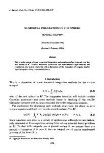
translation with MO2FOR

Fortran source code for QUALIDAES



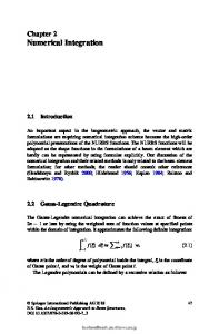
in a certain sense. In general, such an approximation results in a residual rC 6= 0, which in turn leads to unfulfilled constraints, i.e., 0 6= h(xk ,tk ), not even within machine precision. This would lead to the typical difficulties in the numerical integration of higher index DAEs, i.e., instabilities, convergence problems, inconsistencies, or the solution drifts away from the original solution manifold. In order to avoid these problems it is necessary to make sure that the constraints are always satisfied during numerical integration. This can be achieved if the nonlinear system (12) is treated separately such that the next iterate xk satisfies the lower part, i.e., the constraints, exactly or within a prescribed precision, while xk yields a minimal residual in the upper part, i.e., in the differential part. The described numerical approach is implemented in the software package QUALIDAES (QUAsi LInear DAE Solver). This software package is suited for the direct numerical integration of regularized overdetermined model equations and is based on the 3-stage implicit Runge-Kutta method of type Radau IIa of order 5, see [5, 6]. QUALIDAES is integrated as numerical solver into the MPSSim framework. In the current version the user has to provide the model equations already given in overdetermined regularized form (10) formulated as M ODELICA model. Then, using the translator MO2FOR [1] a F ORTRAN source code is generated that can be used to solve the model equations with the solver QUALIDAES. The F ORTRAN source code is automatically compiled and linked to the solver QUALIDAES. In Figure 1 the approach for the numerical treatment of models defined in M ODELICA using MPSSim is illustrated. Note that within this framework, it is not necessary to determine a dynamic (state) selector, since this is achieved automatically within the separated treatment of (12) by its numerical solution, as described above. For a convenient usage also a graphical user interface (GUI) has been implemented in Matlab (see Figure 2) allowing the graphical representation of the obtained numerical results and can be used for further post-processing. DOI 10.3384/ECP140961171

Modelica source code

numerical integration with QUALIDAES

numerical results

Figure 1: Scheme of MPSSim

5

Numerical Example

To show the promising performance of integrating a DAE system using MPSSim with an overdetermined system formulation we have compared the simulation of the simple pendulum equations given in Example 2.1 using MPSSim, MapleSim, Dymola and OpenModelica. In order to have a measurement for the error we include another equation in the system describing the total energy 1 E = m(q21 + q22 ) + mgp2 2 that should be preserved for all t ∈ I and every solution of the system (4). We use a gravitational constant of g = 13.7503716373294544 sm2 to ensure a time period of T = 2s for the motion of the pendulum and a mass of m = 1kg as well as a length of ` = 1m. At first we simulate the system for t ∈ [0s, 100s] with given (fixed) consistent initial conditions p1 (0) = 1, q2 (0) = 0,

p2 (0) = 0,

λ (0) = 0,

q1 (0) = 0, E(0) = 0,

and a prescribed error tolerance of 10−7 (for both the absolute and relative error). In the simulation with MPSSim we solve the overdetermined formulation (4) together with (11) containing all hidden constraints, while the other simulation tools use the original dindex 3 formulation (4) and the index reduction is performed within the tool using different index reduction strategies. The values E(t f ) of the total energy at the final time point t f = 100s together with the required CPU times needed for the integration are listed in Table 1. In Dymola a modified version of the multi-step solver Dassl is used. Here, quite a large number of state selections are required (alternating selecting the

Proceedings of the 10th International ModelicaConference March 10-12, 2014, Lund, Sweden

1175

Efficient Numerical Integration of Dynamical Systems based on Structural-Algebraic Regularization avoiding State Selection

Simulation tool

E(t f )

MPSSim

1.13 · 10−6

0.148s

MapleSim (Rosenbrock)

0.00 · 10−0

4.484s

MapleSim (CK45)

1.50 · 10−5

1.604s

Dymola

2.14 · 10−3

0.890s

−1.60 · 10−3

2.938s

OpenModelica

CPU time

Table 1: Simulation result of the pendulum equation with energy conservation for t ∈ [0s, 100s] Simulation tool

E(t f )

CPU time

MPSSim

1.89 · 10−5

1.364s

MapleSim (Rosenbrock)

5.00 · 10−6

45.358s

MapleSim (CK45)

1.49 · 10−4

15.645s

Dymola

2.14 · 10−2

8.830s

OpenModelica

—

—

Table 2: Simulation result of the pendulum equation with energy conservation for t ∈ [0s, 1000s] are less accurate. The numerical results obtained with MPSSim are accurate within the range of the prescribed error tolerance at low computational costs. However, note that using MPSSim only the costs for the numerical integration of the overdetermined system are measured, while the CPU times of the other tools also contains the costs for index reduction, state selection, projection, and further transformations. Figure 2: Matlab-GUI of MPSSim

6 states p1 and q1 , or p2 and q2 ). In MapleSim we use once the provided solver CK45 suited for semi-stiff problems, which is usually less accurate but faster, and once the Rosenbrock method suited for stiff systems, which yields a higher accuracy at the expense of more required CPU time. Furthermore, the corresponding results obtained for a long time simulation for t ∈ [0s, 1000s] are listed in Table 2. Note that OpenModelica fails to integrate the system in this case. Comparing the obtained results one can see that the projection strategy onto the constraint manifold used within MapleSim yields an accurate numerical solution, while the numerical results obtained with Dymola 1176

Conclusions

In this article we have discussed the efficient and robust numerical simulation of dynamical systems that are modeled with M ODELICA. We have presented a regularization method for quasi-linear DAEs that is based on an overdetermined system formulation that is obtained by adding all hidden constraints explicitly to the original model equation. The information on the hidden constraints can be obtained from a structural analysis of the system. If a structural analysis cannot be applied these information can be obtained in an analytical way. The overdetermined system formulation can then directly be integrated using a specially adapted numerical integrator. The great advantage of the direct discretization of the overdetermined

Proceedings of the 10th International ModelicaConference March 10-12, 2014, Lund, Sweden

DOI 10.3384/ECP140961171

Poster Session

formulation is the fact that it is not necessary to determine a selector analytically in advance and that the number of unknowns in the DAE is not increased. A further advantage of an overdetermined regularization with respect to the numerical integration is the possibility to add solution invariants, e.g., mass, impulse or energy conservation laws, to the constraints, which often stabilizes numerical integration. Performing the state selection within the numerical integrator also allows us to switch between different state selections and also opens the door to handle structure varying system models [11]. Currently, no M ODELICA simulation framework is able to handle overdetermined system formulations. Therefore, a prototype M OD ELICA framework MPSSim is presented that includes a translator MO2FOR that is used to translate an overdetermined system model provided in M ODELICA into F ORTRAN source code which can then be integrated using the software package QUALIDAES. MPSSim is still at an early state of development and will be continuously improved.

Acknowledgements This work has been supported by the European Research Council through Advanced Grant MODSIMCONMP.

References [1] R. Altmeyer and A. Steinbrecher. Regularization and numerical simulation of dynamical systems modeled with Modelica. Preprint 29-2013, Institut für Mathematik, TU Berlin, 2013.

[5] E. Hairer, C. Lubich, and M. Roche. The Numerical Solution of Differential-Algebraic Systems by Runge-Kutta Methods. Springer-Verlag, Berlin, Germany, 1989. [6] E. Hairer and G. Wanner. Solving Ordinary Differential Equations II - Stiff and DifferentialAlgebraic Problems. Springer-Verlag, Berlin, Germany, 2nd edition, 1996. [7] P. Kunkel and V. Mehrmann. Index reduction for differential-algebraic equations by minimal extension. Zeitschrift für Angewandte Mathematik und Mechanik, 84(9):579–597, 2004. [8] P. Kunkel and V. Mehrmann. DifferentialAlgebraic Equations. Analysis and Numerical Solution. EMS Publishing House, Zürich, Switzerland, 2006. [9] S. Mattsson and G. Söderlind. Index reduction in differential-algebraic equations using dummy derivatives. SIAM Journal on Scientific and Statistic Computing, 14:677–692, 1993. [10] C.C. Pantelides. The consistent initialization of differential-algebraic systems. SIAM Journal on Scientific and Statistic Computing, 9:213–231, 1988. [11] P. Pepper, A. Mehlhase, Ch. Höger, and L. Scholz. A compositional semantics for Modelica-style variable-structure modeling. In P. Fritzson F.E. Cellier, D. Broman and E.A. Lee, editors, 4th International Workshop on Equation-Based Object-oriented Modeling Languages and Tools (EOOLT 2011), number 56 in Linköping Electronic Conference Proceedings, pages 45–54, Zurich, Switzerland, September 2011. September 5, 2011.

[2] K.E. Brenan, S.L. Campbell, and L.R. Petzold. Numerical Solution of Initial-Value Problems in Differential Algebraic Equations, volume 14 of Classics in Applied Mathematics. SIAM, [12] J. Pryce. A simple structural analysis method Philadelphia, PA, 1996. for DAEs. BIT Numerical Mathematics, 41:364– 394, 2001. [3] C.W. Gear. Differential-algebraic equation index transformations. SIAM Journal on Scientific and [13] L. Scholz and A. Steinbrecher. A combined Statistic Computing, 9:39–47, 1988. structural-algebraic approach for the regularization of coupled systems of DAEs. Preprint 30[4] E. Griepentrog and R. März. Differential2013, Institut für Mathematik, TU Berlin, 2013. Algebraic Equations and Their Numerical TreatAnalysis of quasi-linear ment, volume 88 of Teubner-Texte zur Mathe- [14] A. Steinbrecher. differential-algebraic equations. Preprint 11matik. BSB B.G.Teubner Verlagsgesellschaft, 2006, Institut für Mathematik, TU Berlin, 2006. Leipzig, 1986. DOI 10.3384/ECP140961171

Proceedings of the 10th International ModelicaConference March 10-12, 2014, Lund, Sweden

1177

Efficient Numerical Integration of Dynamical Systems based on Structural-Algebraic Regularization avoiding State Selection

[15] A. Steinbrecher. Numerical Solution of QuasiLinear Differential-Algebraic Equations and Industrial Simulation of Multibody Systems. PhD thesis, Technische Universität Berlin, 2006. [16] A. Steinbrecher. Deflating type regularization method for quasi-linear differential-algebraic equations. Preprint, Institut für Mathematik, TU Berlin, 2013. In preparation.

1178

Proceedings of the 10th International ModelicaConference March 10-12, 2014, Lund, Sweden

DOI 10.3384/ECP140961171