illustrate the significant improvement over existing path-based matching methods. .... diffusion values follow directions perpendicular to image gradients. Valentinotti and ...... ground truth than the matching obtained by Sun's method. The.
(JOURNAL NAME), VOL. (VOLUME), NO. (NUMBER), (MONTH) (YEAR)
1
Efficient Path-Based Stereo Matching With Sub-pixel Accuracy Arturo Donate1 , Ying Wang1 , Xiuwen Liu1 , and Emmanuel Collins2
Abstract—This paper presents an efficient algorithm to achieve accurate sub-pixel matchings for calculating correspondences between stereo images based on a path-based matching algorithm. Compared to point-by-point stereo matching algorithms, pathbased algorithms resolve local ambiguities by maximizing the cross correlation (or other measurements) along a path, which can be implemented efficiently using dynamic programming. An effect of global matching criterion is that cross correlations at all pixels can contribute to the criterion; since cross correlation can change significantly even with sub-pixel changes, to achieve sub-pixel accuracy, it is no longer sufficient to first find the path that maximizes the criterion at integer pixel locations and then refine to sub-pixel accuracy. In this paper, by writing bilinear interpolation using integral images, we show that cross correlations at all sub-pixel locations can be computed efficiently and thus lead to a sub-pixel accuracy path based matching algorithm. Our results show the feasibility of the method and illustrate the significant improvement over existing path-based matching methods. Index Terms—Computer vision, disparity, stereo, path-based matching, integral image, normalized cross correlation, sub-pixel accuracy, bilinear interpolation
I. I NTRODUCTION
T
HE use of stereo images in computer vision is crucial for applications requiring depth perception [1]. In order to be useful, stereo vision algorithms rely on the ability to perform accurate point correspondence between the image pair [2]. This correspondence is defined as the problem of finding the accurate location of the same point in the scene in a pair of stereo images. So for a given pixel, corresponding points must describe the same content, although their image coordinates may differ. It is useful to note that these corresponding points may also be used for motion estimation, as well as many other applications. Stereo correspondence methods can be divided into two main types: region-based and feature-based methods. Regionbased methods attempt to find corresponding points by matching intensity values across images. These searches are typically performed within local image windows in both images. In some cases, if the geometry of the scene is previously known, the search can be performed across lines as defined by the epipolar constraint [3]. Feature-based methods typically rely on matching more distinctive features. Such features are typically assumed to have some higher level meaning (as opposed to image points), and thus are assumed to be more Manuscript received MONTH DAY, YEAR; revised MONTH DAY, YEAR. The authors are with the Department of Computer Science at Florida State University1 , and the Department of Mechanical Engineering at the FAMUFSU College of Engineering2 , Tallahassee, FL, 32306 USA. (email: {donate, ywang, liux}@cs.fsu.edu)
stable. Several types of image features can be used. Harris corners [4], Canny edges [5], or even SIFT points [6] would typically provide features that are likely to be easily located in stereo image pairs. To calculate a dense matching, regionbased methods are widely used. A common approach for solving the correspondence problem is to match the local windows using normalized cross correlation as well as other matching criteria. This regionbased method yields results with pixel-level accuracy. In order to achieve accuracy at a sub-pixel level, typically a second order polynomial is used to fit matching scores in a local neighborhood [7]. One of the intrinsic limitations of such region-based matching methods is their inability to resolve local ambiguities effectively. For example, for a given image point, there can often be multiple matching candidate points in the candidate region of the corresponding image. These multiple candidate points often arise from situations with low texture variations, as well as other factors. In addition, local deformations may cause the correct matching point not to be the local maximum, causing many of the algorithms dependent on local maxima to fail. To overcome the local ambiguities and achieve more robust matching, a more global matching criterion may be used. Sun [8] poses the stereo matching problem as an optimization of the total cross correlation scores over a surface through a 3D cross correlation volume (whose dimensions are given by height, width, and the disparity range of a region). The matching is solved efficiently using a two-stage dynamic programming algorithm. This algorithm attempts to maximize cross correlation scores along paths in the 3D cross correlation volume. It is important to note that by using a global matching criterion, accurate cross correlation values are needed at all locations since they affect the optimal path estimation (and thus the matching). Since cross correlations can change significantly even at the sub-pixel level, correlation measurements must be calculated with sub-pixel accuracy in order to achieve an optimal stereo matching. In his work, Sun [8] performs sub-pixel measurements as a post processing stage by fitting a quadratic function in a neighborhood. In this paper, we aim to show that cross correlation values calculated with sub-pixel accuracy provide a significant improvement to the path-based stereo matching, and this is supported by experimental results. These measurements can be performed efficiently by exploiting certain aspects of the calculations and employing the use of integral images [9], [10]. The rest of the paper is organized as follows. Section II provides a review of the recent literature in the area. In Section III, we summarize the path-based stereo matching algorithm [8]
(JOURNAL NAME), VOL. (VOLUME), NO. (NUMBER), (MONTH) (YEAR)
and in Section IV we show how the sub-pixel accuracy can be incorporated efficiently using integral images; note that while Sun [8] also performs sub-pixel matching, it is done after the path matching. As shown by our results in Section V, our algorithm improves the performance significantly by having more accurate path matching. Section VI concludes the paper. II. BACKGROUND Although stereo matching is one of the classical problems in computer vision, its focus is presets in other areas such as medical imaging, computer graphics, and image processing. A considerable amount of work has been done on this specific subject over the last 30 years. More specifically, the past decade has brought a plethora of proposed methods for solving this correspondence problem. Mansouri et. al. [11] presented an algorithm for calculating disparity images based on selective image diffusion so that diffusion values follow directions perpendicular to image gradients. Valentinotti and Taraglio [12] presented a stereo matching method based on phase difference. The method involves shifting one of the two phase signals, in order to use a phase difference approach. Since errors associated to phase differences increase very rapidly as changes in disparity increase, this method is only able to handle stereo pairs with very small disparities. Kolmogorov and Zabih [13] proposed an algorithm for calculating point correspondence using graph cuts that does performs well when dealing with occlusions. Szeliski and Scharstein [14] proposed an algorithm that derives a matching cost from reconstructed image signals, then assigns disparity values based on a symmetric matching process that incorporates sub-pixel information. Kim et. al. [15] presented a framework that incorporates stereo imagery for interaction between real and augmented worlds. Here, they perform stereo matching by first dividing the input images into separate regions. Afterwards the matching is performed using the mean absolute distances criterion. Kim and Chung [16] presented an algorithm for stereo matching which successfully handles large depth discontinuities by using variable windows on the images. The correlation between candidate points is determined using normalized cross correlation, as well as sum of squared differences. Sub-pixel measurements are used to reduce occasional local deformations which may rise due to the variable windows. Brockers et. al. [17] poses the problem of stereo matching as an optimization one. For a given pixel, a range of possible disparities is first assigned. Then, the best disparity value is calculated by optimizing a global cost function, taking into account stereoscopic properties as well as similarity measurements, in order to produce a dense matching. Kim [18] proposed a stereo matching algorithm which handles depth discontinuities as well as smooth, texture-less regions. Variable windows are used to handle the large discontinuities, and an intensity gradient-based similarity is defined to reduce the smoothness of smooth, texture-less regions. Similarity measurements are performed using a correlation function based on voxel components. Rosenberg et. al. [19] presented a system for real-time stereo using programmable graphics hardware.
2
The system employs a matching algorithm originally proposed by Hirscmuller [20]. This semi-global matching algorithm uses dynamic programming to work across an image in n directions while storing partial results. For each pixel, the system uses the cost and disparity range of each pixel to find the shortest path though the disparity range ending at d. This shortestpath disparity becomes the final disparity value for the given location. Muquit et. al. [21] proposed a 3D reconstruction system for multi-camera passive stereo. The system relies on an efficient phase-based stereo matching technique to generate a matching. Using a 2D Discrete Fourier Transform, the system employs a coarse-to-fine search along with outlier detection and a phaseonly correlation function to estimate the peak position via function fitting. This technique delivers a dense matching of arbitrary 3D shapes. Delon and Roug´e [22] study the problem of stereopsis in cases where the baseline is relatively small. They proposed a multi-scale matching algorithm that employs the use of block matching. Their study shows that it is possible to predict where reliable matchings will occur, within the realm of small baseline stereo. Ulusoy and Hancock [23] present a feature-based method for generating sparse disparity maps from stereo images. Steerable filters are first used to extract features from the images, then phase similarity is used to establish correspondences. Phase differences between established corresponding features are then used to fine tune results and achieve subpixel accuracy. Liang et. al. [24] presented a 3D reconstruction method to extract depth information from a tele-robotic welding environment. Using stereo images, they combine the use of stereo vision algorithms along with structured light in order to perform accurate reconstructions. The simple region-based matching is performed using a sum of squared differences criterion. Zhao et. al. [25] proposed a novel approach to solve for a matching by using double harris corner detectors. This feature-based method uses Harris corner detection to first locate a corner feature, then again to adjust its location with sub-pixel accuracy. The matching is performed using cross correlation, and uses characteristics of the corners in order to limit the candidate matches in a given search window. In the next section, we discuss in detail the path-based matching algorithm proposed by Sun [8]. III. PATH - BASED S TEREO M ATCHING The research work presented here was inspired by the work of Sun [8]. There Sun presents a dynamic programming algorithm which uses rectangular subregioning and maximum surface techniques in order to perform path-based matching. This section describes the different parts of his proposed approach. A. Rectangular Subregioning Initially, the images are segmented into subregions in order to reduce computation time, as well as memory requirements of the system. In a given stereo image pair, different image points may have disparity values that lie within very different ranges. The aim of the subregioning step is to segment the
(JOURNAL NAME), VOL. (VOLUME), NO. (NUMBER), (MONTH) (YEAR)
3
image in a way such that each point in a given subregion contains a similar range of disparity values. For a given image point location, the goal is now to determine the disparity value within the specified disparity range which yields the optimal normalized cross correlation measurement. A 3D volume of size W × H × D can be constructed from the correlation coefficients, where W and H are the subregion dimensions and D is the size of the disparity range. Since the subregioning process segments the images into regions containing similar disparity ranges, each region can then be viewed as a smaller 3D volume of size Wi × Hi × Di , where Wi ≤ W and so on. Each subregion is performed as follows. First, the image is divided evenly into a set number of rows. Adjacent rows are compared and merged using a criterion of minimizing overall computational complexity. Next, the resulting regions are divided into a set number of horizontal columns. A similar merging process is repeated until there are no more columns that can be merged. The resulting subregions are the output of the rectangular subregioning process. B. Matching Algorithm After the rectangular subregioning process, a 3D volume of correlation coefficients can be created for every point (i, j, d) in the volume, where i, j are the row and column indices obtained from the pixel coordinates, and d is the possible disparity values defined by the disparity range (which may vary across different subregions in order to decrease computational costs). In other words, the value at coordinate (i, j, d) within the volume is the zero-mean normalized cross correlation value between windows in the stereo images f and g using a disparity value of d . Each window is of size M × N , and is centered at location (i, j) . This normalized cross correlation is defined by Equation 1 as: C(i, j, d) = p
covij,d (f, g) p varij (f ) × varij,d (g)
(1)
where (i, j) are the row and column indices of the 3D correlation volume (i.e., pixel location), and d is the possible disparity value. Here, varij (f ) refers to the variance within a window centered at (i, j) of the image f , and covij,d (f, g) refers to the covariance between the windows of the left and right images. The disparity term d is obtained from the given disparity range in the subregion, corresponding to a shift of the window along the epipolar lines. Since the epipolar lines may not always be available, rectified images are used (i.e., a shift along the epipolar lines corresponds to a shift along the y axis of the image). In order to compute correlation values efficiently, Sun employs the use of box filtering [8], [26], [27]. Given this 3D volume of correlation coefficients, Sun employs a two stage dynamic programming algorithm to find the best surface across the volume and obtain a smooth set of disparity values. The first stage of the dynamic programming algorithm is to separate the volume vertically and calculate an intermediate 3D volume in the vertical direction for each vertical section. Given the original 3D correlation volume C,
the intermediate 3D volume Y is calculated according to the equation: Y (i, j, d) = C(i, j, d) + max Y (i − 1, j, d + t), t:|t|≤p
(2)
where p determines the number of local values to be considered. For example, when p = 1, the three locations d − 1, d, and d + 1 are considered. In other words, at a given vertical level, only the values that are a distance p from the previous value (in both directions) are considered. The algorithm begins on the highest vertical section and works its way down. In this initial step, i − 1 will be undefined, so it is set to zero. Therefore, when i = 0, Y (0, j, d) = C(0, j, d)
(3)
so that the very top vertical section is identical to the top section of the 3D volume C. By the end of the first stage of this dynamic program, the bottom vertical section of the intermediate volume Y contains a summation of the maximum correlation values. Note that the stereo pair is assumed to be rectified, i.e., the corresponding row in the left image matches with that of the right image and thus the disparity is specified by d. The 3D volume of Y then contains the maximum summation of correlation coefficients in the vertical direction. The second stage of the algorithm works in the horizontal direction calculating the path from the left side to the right side of the volume that maximizes the summation of Y ’s along the path. First, the algorithm begins by selecting the bottom slice of the intermediate volume Y . It begins at the bottom slice because this is where the correlation values are accumulated. Using a shortest path algorithm similar to the one used in the first stage, the shortest path along the bottom slice of the intermediate volume Y is calculated (this bottom slice has dimensions W × D). For the next iteration, the algorithm calculates the shortest path in the next level above the current one, until it finds a path at all levels of Y . For each level (not including the bottom level), the shortest path in a given level is constrained to be at a distance no larger than p from the previous shortest path. The value of p was previously defined in Equation 2, and is typically kept at or near 1 in order to keep computational costs low. This method proposed by sun [8] leads to an efficient pathbased matching algorithm. In order to increase the quality of the matching, sub-pixel accuracy is performed as a post processing step by the use of a quadratic function over pixels in a neighborhood. The author fits a second degree curve to the correlation coefficients around the neighborhood of a pixel, and use the extrema of the curve to solve for the disparity. This additional step improves the quality of the results over only using pixel values at integer locations. However, this sub-pixel accuracy matching is not optimal, as the obtained paths may not be optimal if we consider sub-pixel cross correlations. In addition, the quadratic functions used are not sufficient for bilinear interpolation. IV. S TEREO M ATCHING WITH S UB - PIXEL ACCURACY Our goal is to achieve a dense matching accurate to the sub-pixel level while maintaining a low computational cost,
(JOURNAL NAME), VOL. (VOLUME), NO. (NUMBER), (MONTH) (YEAR)
4
in order to obtain an optimal matching efficiently. As in the work by Sun [8], we assume that the input stereo pair is rectified, i.e., the matching row is within one row from the corresponding row. Unlike Sun’s approach, however, our proposed method incorporates the use of sub-pixel measurements into the correlation calculation, effectively making the correlation coefficients more accurate, and allowing the pathbased matching to achieve a more accurate matching. In order to perform such computations efficiently, we employ the use of integral images. A. Correlation Measurements As in the work by Sun [8], we also adopt normalized cross correlation as given in Equation (7). Given a left image f , a right image g, and a pixel location in the left image f (x0 , y0 ), the goal is to compute the optimal pixel location in the right image g corresponding to the point f (x0 , y0 ) in the left image. In order to achieve this, normalized cross correlation is used as a similarity measure on a window of size of (2M + 1) × (2N + 1) on the right image, for a displacement (u0 , v0 ). The value obtained from the similarity measure will then be used with the path based matching proposed by Sun [8]. Here the first dimension (e.g., x, u, x0 , M ) refers to the column of the image, and the second dimension (e.g., y, v, y0 , N ) refers to the row of the image. To define the normalized cross correlation, we first define the mean of the window in the left image as i=M j=N 1 X X ¯ f (x + i, y + i) f (x, y) = S
using integral images as well as the mean and variance of a local window. For the variance, note that f¯¯(x, y) is defined as: X (1/S)( f 2 (x0 + i, y0 + j)) − (f¯(x, y))2 , (9) i,j
and thus it can also be done efficiently using an integral image with pixel values squared. B. Integral Images Originally proposed by Viola and Jones [9], an integral image is an intermediate representation of an image that aids in solving certain problems in computer vision. It is essentially an additive representation of an original image where the value at a given location is equal to the sum of the pixel values at locations to the left and above the current index location. Formally it is defined as I(x, y) =
y x X X
O(i, j),
(10)
i=0 j=0
where O is the original image and I is the integral image being calculated. As described by Viola and Jones [9], they can be computed in one pass over the original image.
(0, 0)
a
b
d
c
(4)
i=−M j=−N
and the variance of the window as i=M X j=N X 1 f (x + i, y + i)2 − f¯(x, y)2 (5) f¯¯(x, y) = S i=−M j=−N
where C is defined as: S = (2 × M + 1)(2 × N + 1).
(6)
To be specific, let f¯(x, y) and g¯(x, y) be the mean of the left and right windows centered at (x, y) and of size M × N . Similarly, let f¯¯(x, y) and g¯(x, y) be the variance of the left and right windows. We can define the normalized cross correlation (NCC) between the left image window at (x0 , y0 ) and the right image window at (x0 + u, y0 + v) as N CC(x0 , y0 , u, v) = P ˆ i,j f (x0 + i, y0 + j)g(x0 + u + i, y0 + v + j) q , (7) S f¯¯(x0 , y0 )g¯(x0 + u, y0 + v) where fˆ is defined as: fˆ(x0 + i, y0 + j) = f (x0 + i, y0 + j) − f¯(x0 , y0 ),
(X, Y) Fig. 1. Integral image. The sum of the shaded region can be computed from the indices of the four points.
The main benefit for such a data structure is that any given rectangular sum can be calculated from four references to the integral image. These sums only require four lookups to the integral image. Assume we have an integral image I and four points in this image which define a square: a, b, c, d. If the square is defined as in Figure 1, then the sum of the values within that square is calculated as sum(a, b, c, d) = I(c) + I(a) − I(b) − I(d)
(11)
(8)
and the summation for i is from −M to M and j from −N to N (also in subsequent equations). As pointed out in [8], [9], for a fixed u and v, the summations can be done efficiently
where I(x) corresponds to the value of the integral image at location x. Integral images have been used extensively in solving realtime computer vision problems. Viola and Jones [9] used
(JOURNAL NAME), VOL. (VOLUME), NO. (NUMBER), (MONTH) (YEAR)
5
(a)
(b)
(c) Fig. 2. Disparity map for stereo pairs (left images) using the method in [8] (middle images) and the proposed method (right images). (a) A baseball pair. (b) A park meter scene. (c) An outdoor ground.
them to solve the problem of face recognition in real time. Frintrop et. al. [28] use integral images to aid in fast image feature computation in their real-time visual attention system. Kisacanin [29] uses integral images in embedded systems to solve complex computations efficiently, and describes optimization methods that allow acceptable execution costs in embedded processors by taking advantage of recursion and double buffering techniques. Bay et. al. [10] used integral images in order to speed up the computation of their robust feature extraction algorithm. In this article, we will show that integral images can also be used to compute normalized cross
correlation values of stereo images with sub-pixel accuracy in an efficient manner. C. Bilinear Interpolation Due to the nature of digital images, pixel values are only defined at integer locations. Therefore, in order to perform effective sub-pixel measurements, we propose the use of bilinear interpolation. It is used to compute the value of a function at an unknown (x, y) coordinate. Given the values for the surrounding coordinates at locations (x + 1, y), (x − 1, y), (x, y+1), and (x, y−1), linearly interpolating in each direction
(JOURNAL NAME), VOL. (VOLUME), NO. (NUMBER), (MONTH) (YEAR)
6
allows the estimation of the value at (x, y) computed as a weighted average of the four known points. This interpolation allows us to estimate the value of an image at sub-pixel locations (corresponding to non-integer coordinates previously undefined in the image).
the bilinear interpolation, we can express the right image g as:
Bilinear interpolation has been widely used to solve computer vision and image processing problems in the literature. Kim and Kim [30] proposed a system that uses image measurements to detect scratches in film, then employs the use of bilinear filtering in order to sample the surface of the image and recover the scratched regions. Velden et. al. [31] propose the use of bilinear filtering for filling in gaps from high resolution medical scans obtained using 3D-filtered backprojection strategies. Fahmy [32] proposed an architecture for efficient calculation of bilinear filtering techniques on field programmable gate arrays.
(12)
g(x + s, y + t) (g(x, y)(1 − s) + g(x + 1, y)s) (1 − t) + (g(x, y + 1)(1 − s) + g(x + 1, y + 1)s) t = g(x, y)(1 − s)(1 − t) + g(x + 1, y)s(1 − t) + g(x, y + 1)(1 − s)t + g(x + 1, y + 1)st = [g(x, y) − g(x + 1, y) − g(x, y + 1) + g(x + 1, y + 1)]st + [−g(x, y) + g(x + 1, y)] s + [−g(x, y) + g(x, y + 1)] t + g(x, y). =
D. Correlation Measurements at the Sub-pixel Level Using bilinear interpolation as defined by Equation 12 along with normalized cross correlation as defined by Equation 7, we can compute correlation measurements for points previously undefined at sub-pixel locations. The correlation value between two such points can change significantly, even for fractional changes in u and v. In order to make the path matching algorithm effective at the sub-pixel level, we define Nd CC(x0 , y0 , u, v) as: = arg max−.5≤s≤.5, −.5≤t≤.5 N CC(x o0 , y0 , u + s, v + t) n = maxk=1,···,4 Nd CC k (x0 , y0 , u, v) , (13) assuming that u and v will be integer values. For each value of k, we define Nd CC k as
Fig. 3.
Illustration of sub-pixel location as calculated in the right image.
Since images are discrete in nature, we define the bilinear interpolation for 0 ≤ s, t ≤ 1 in the right image only, as illustrated in Figure 3. In other words, given a pixel location in the left image, we would like to find the sub-pixel location in the right image that gives an optimal match. According to
Nd CC 1 (x0 , y0 , u, v) = arg max−0.5≤s≤0, −0.5≤t≤0 N CC(x0 , y0 , u + s, v + t), Nd CC 2 (x0 , y0 , u, v) = arg max0≤s≤0.5, −0.5≤t≤0 N CC(x0 , y0 , u + s, v + t), Nd CC 3 (x0 , y0 , u, v) = arg max−0.5≤s≤0, 0≤t≤0.5 N CC(x0 , y0 , u + s, v + t), Nd CC 4 (x0 , y0 , u, v) = arg max0.0≤s≤0.5, 0≤t≤0.5 N CC(x0 , y0 , u + s, v + t). (14) Here N CC(x0 , y0 , u + s, v + t) are defined using bilinear interpolation. The central problem is how to compute Nd CC k (x0 , y0 , u, v) (for all k = 1, · · · , 4) efficiently. Clearly, a brute force implementation will be computationally expensive and undesirable. Instead, we exploit certain properties of these calculations through the use of integral images in order to compute Nd CC k efficiently for all values of k. In the following example, we show how the computation can be done for Nd CC 4 , but the same basic algorithm can be used for the three other values of k. As given in Equation (7), in order to compute Nd CC 4 (x0 , y0 , u, v), we need to compute the summation of images with pixel values squared. Let x1 y1 x2 y2
= x0 + u = y0 + v = x0 + u + 1 = y0 + v + 1.
(15)
(JOURNAL NAME), VOL. (VOLUME), NO. (NUMBER), (MONTH) (YEAR)
7
Using bilinear interpolation, we have P g(x1 + i + s, y1 + j + t)2 Pi,j = i,j [g(x1 + i, y1 + j)(1 − s)(1 − t) +g(x2 + i, y1 + j)s(1 − t) +g(x1 + i, y2 + j)(1 − s)t 2 +g(x2 + i, y2 + j)st hP ] i 2 = (1 − s)2 (1 − t)2 g(x + i, y + j) 1 1 i,j hP i 2 +s2 (1 − t)2 g(x 2 + i, y1 + j) i,j hP i 2 +(1 − s)2 t2 g(x + i, y + j) 1 2 i,j hP i 2 +s2 t2 g(x 2 + i, y2 + j) i,j hP i +C1 g(x + i, y + j)g(x + i, y + j) 1 1 2 1 hPi,j i +C2 i,j g(x1 + i, y1 + j)g(x1 + i, y2 + j) hP i +C3 g(x + i, y + j)g(x + i, y + j) 1 1 2 2 hPi,j i +C4 i,j g(x2 + i, y1 + j)g(x1 + i, y2 + j) hP i +C5 g(x + i, y + j)g(x + i, y + j) 2 1 2 2 hPi,j i +C6 i,j g(x1 + i, y2 + j)g(x2 + i, y2 + j) ,
V. E XPERIMENTAL R ESULTS
(16)
A. Initial Results
where C1 C2 C3 C4 C5 C6
= 2(1 − s)s(1 − t)2 = 2(1 − s)2 (1 − t)t = 2(1 − s)s(1 − t)t = 2(1 − s)s(1 − t)t = 2s2 (1 − t)t = 2(1 − s)st2 .
(17)
As the derivation of Equation 16 breaks down the original P equation into a series of summations, these i,j terms can all be computed very efficiently via integral images, in the same manner as described in Section IV-B. In order to compute Nd CC 4 (x0 , y0 , u, v), four additional integral images are required: g(x, y)g(x + 1, y), g(x, y)g(x, y + 1), g(x, y)g(x + 1, y + 1), g(x, y + 1)g(x + 1, y + 1).
(18)
For g¯(x1 + s, y1 + t), we have
=
g¯(x1 + s, y1 + t) (1 − s)(1 − t)¯ g (x1 , y1 ) +s(1 − t)¯ g (x1 + 1, y1 ) +(1 − s)t¯ g (x1 , y1 + 1) +st¯ g (x1 + 1, y1 + 1).
Here we provide several examples to illustrate the results obtained by our proposed algorithm. Since our method is an extension of the work by Sun [8], we provide direct comparisons between results generated by his method and results generated by ours. The results presented here show the feasibility of our method, as well as illustrate the improvements over the original algorithm. All datasets were either obtained from Sun’s publication [8], the stereo image database of Scharstein and Szeliski [33], or generated by us with a Bumblebee stereo camera. For some of the experiments presented here, we do not show the entire image frame in our examples. Rather, we show cropped regions of the results in order to better illustrate the finer differences obtained between the two algorithms.
(19)
By combining Equations (16) and (19), we are able to compute normalized cross correlation values accurate to the sub-pixel level. The calculation is done efficiently by solving the summation terms using integral images. As all the integral images only need to be computed once, they will not increase the computational complexity in a significant way for a given stereo pair.
This first set of results shown in Figures 2 and 4 were initially published in our preliminary paper [34]. The first example illustrated in Figure 2(a) presents results using stereo images obtained from the test data of Scharstein and Szeliski [33]. The left image shows one of the stereo images, a baseball against a noisy background. The second image shows the disparity map obtained by Sun’s algorithm. Notice that the algorithm obtains a good matching of the image points. The rightmost image is the disparity image obtained with our algorithm, incorporating our sub-pixel measurements. Notice that the boundaries of the ball are sharper and better defined than the ones provided by Sun’s algorithm. This example shows a clear advantage of our sub-pixel measurement approach. The second example in Figure 2(b) presents an outdoor scene from the test data of Scharstein and Szeliski [33]. The disparity image generated by Sun’s algorithm presents an accurate estimate of the scene’s depth, but contains some noise, particularly in areas of low texture. Our disparity image, however, obtained sharper boundaries and smoother disparity areas. The third example illustrated in Figure 2(c) presents an image of the ground taken from a 45o angle such that the top region of the image represents the part of the ground that is furthest from the stereo camera. As before, Sun’s algorithm provides an accurate estimate of the depth in the scene. Our results, however, provide a smoother disparity image with correct depth estimation. This example illustrates the path-based matching algorithm’s ability to find smooth paths along the intermediate 3D volume of correlation coefficients when these coefficients are obtained with sub-pixel accuracy. Although the result of Sun’s method is smooth, it is still outperformed by our approach. The fourth example illustrated in Figure 4(a) combines the image of the third experiment (illustrated in Figure 2(c)) with the rear-view mirror of a car in the foreground. As in the previous cases, Sun’s algorithm does a good job of recovering scene depth. Our disparity image, however, is able to recover better boundaries between the foreground object (car) and the background (ground), as well as provide a smoother disparity map overall. It also appears to perform slightly better in recovering the depth of the ground in relation to the car.
(JOURNAL NAME), VOL. (VOLUME), NO. (NUMBER), (MONTH) (YEAR)
8
(a)
(b) Fig. 4.
Two additional disparity map examples. See Fig. 2 for figure caption. (a) Part of a car and ground. (b) A stereogram pair.
The fifth example presented is illustrated in Figure 4(b). The input images were a stereogram pair obtained from the publication by Sun [8]. The results show that although Sun’s method provides a good disparity map, our results show more accurate boundaries around the edges of the squares, as well as overall smoother measurements inside each region. B. Accuracy Measurements As shown in Section V-A, our proposed approach of including sub-pixel measurements into the correlation calculations exhibits clear advantages over the previously published work by Sun [8]. Our approach shows improvements in finding accurate boundaries between the objects in the scene, but sometimes may sacrifice small image details. In this section, we perform a matching on images obtained from the data set provided by Scharstein and Szeliski [33]. We compare results of our method as well as Sun’s previously published method against ground truth images. Distances between the disparity images and the ground truth images are quantified using wellknown error metrics. This set of experiments contains comparison results for seven different data sets, illustrated in Figures 5 and 6. For each row in the figures, four images are displayed; the leftmost image is one of the original stereo images; the second image is the ground truth disparity image; the third image is Sun’s disparity matching; finally, the fourth image is our algorithm’s
result for disparity matching. Each experiment was calculated over an arbitrary image region of pixel size 100 × 100. Only pixels for which occlusion does not occur were taken into consideration (occluded pixels are displayed as black in the ground truth image). Although the path-based algorithm does a good job of estimating disparity values for regions where occlusion occurs, we decided to only take into account regions for which the ground truth value is known. Both the disparity images and the ground truth images were normalized prior to any comparison. In order to quantify the comparison results, three different error metrics were used: sum of square differences (SSD), root mean squared (RMS), and bad matching pixels (BMP) [35]. Each is defined as follows: P 2 SSD = N1 x,y (dI (x, y) − dT (x, y)) � P �1 2 2 RM S = N1 x,y |dI (x, y) − dT (x, y)| (20) P BM P = N1 x,y (|dI (x, y) − dT (x, y)| > δd ) where dI is the calculated disparity image, dT is the ground truth disparity image, and δd is a disparity error tolerance (i.e., allowed error threshold). In the following experiments, an error tolerance of δd = 0.05 was used. The quantified results of comparing each of the disparity images against the ground truth are shown in Table I. These error measurements illustrate the distance between each disparity image and its corresponding ground truth. Visual analysis of
(JOURNAL NAME), VOL. (VOLUME), NO. (NUMBER), (MONTH) (YEAR)
9
(a) Baby
(b) Bowling
(c) Dolls Fig. 5.
Resulting Disparity Comparisons
the disparity images illustrates that our results almost always look far more accurate than Sun’s original method. Our method is able to provide a matching that is closer overall to the ground truth than the matching obtained by Sun’s method. The error measurements show that for the first three experiments presented (Figures 5(a)-(c)), we achieve results significantly closer to the ground truth. This first example in Figure 5 shows a partial view of a doll against a textured background. The arm of the doll is more clearly visible in our result than Sun’s, and the object distances more closely match the ground truth. The second example shows the top of a bowling pin in front of a bowling ball, with a partially-textured background. Here, both methods achieve good results for the bowling pin. The ball is a bit more clearly defined in our method. The background is also more accurately defined in our method, whereas Sun’s method is unsuccessful in determining the proper disparity. The final example of Figure 5 shows a series of dolls at different depths. The bear in the foreground is much more clearly defined in
our method. Also, the boundary between the far doll and the background, although very small, is detected by our method, whereas Sun’s approach fails to detect this boundary. The first example in Figure 6(a) shows the top corner of a lamp shade against a texture-less background. Both disparity maps for this image look similar, but our map is able to calculate a more accurate boundary between the foreground and background objects. It is also able to obtain a more accurate disparity value for the foreground object, closer to the values of the ground truth image. The next example in Figure 6 shows the lower corner of a lamp shade (in the upper left corner of the image), a section of a pillow, part of a hat, and a texture-less background. Neither of the methods achieved accurate boundaries for the disparity map, but our method was at least able to calculate accurate object distances. The third example in Figure 6(c) shows a post coming from the right side of the window, against a partially textured background. Interesting to note, although our disparity map appears visually closer to the ground truth, Sun’s method
(JOURNAL NAME), VOL. (VOLUME), NO. (NUMBER), (MONTH) (YEAR)
10
TABLE I E RROR VALUES FOR F IGURES 5 AND 6 DATA Baby Bowling Dolls Lamp Hat Teddy Aloe
Algorithm Sun Ours Sun Ours Sun Ours Sun Ours Sun Ours Sun Ours Sun Ours
SSD 0.0239 0.0174 0.1373 0.0460 0.0246 0.0200 0.0468 0.0449 0.0644 0.0377 0.0189 0.0192 0.0268 0.0351
RMS 0.1544 0.1320 0.3706 0.2146 0.1568 0.1414 0.2164 0.2119 0.2538 0.1942 0.1375 0.1385 0.1638 0.1874
BMP 0.1286 0.0941 0.2975 0.1528 0.1368 0.0891 0.2001 0.1549 0.2159 0.1409 0.1119 0.0895 0.1120 0.1340
0.14
Normalized SSD Error
Data
Ours Sun
0.12 0.1 0.08 0.06 0.04 0.02 0 1
2
3
4
5
6
7
Data Set
(a) SSD Error
C. Drawbacks and Limitations Although our proposed method is capable of obtaining excellent results efficiently, it does not always obtain a perfect or acceptable matching. Analyzing the images visually, our method successfully provides smaller errors than Sun’s algorithm, as well as better boundaries between the objects in the scene. Our disparity images also have a smoother appearance along surfaces, reducing noise in sections of the disparity images caused by incorrect matches. Our method, however, sometimes sacrifices the smaller visual details of the scene. At times, texture-less regions may cause the path-based matching step to generate errors in the matching. Such an error is illustrated in Figure 5(b). In our disparity image, near the top of the bowling ball (near the right border of the image), one can see errors in the disparity. It does not always occur, but at certain times the path-based approach will get lost in texture-less regions. Notice that Sun’s result contains the same error. The error is more prominent in ours due to the sub-pixel accuracy.
Normalized RMS Error
0.4 Sun Ours
0.35 0.3 0.25 0.2 0.15 0.1 0.05 0 1
2
3
4
5
6
7
Data Set
(b) RMS Error
0.3 Ours Sun
Normalized BMP Error
achieved smaller error values for the SSD and RMS metrics. Our method achieved a smaller error according to the BMP error, however. In the final example illustrated in Figure 6(d), Sun’s method provided results that were closer to the ground truth according to all three error measurements. This example shows that sub-pixel accuracy does not improve results 100% of the time. This may be caused by either sub-optimal segmentation of regions in the subregion step, or noise in the images. Either of these cases may introduce errors in the correlation process which, when large enough, may cause the path-based algorithm to calculate an incorrect disparity value. However, from our experiments we observe that such errors are not a common occurrence. The error measurements for all these experiments are illustrated in the graphs of Figure 7. The vertical axis of the graph represents the error values, and the horizontal axis represents each of the seven experiments in Table I (also illustrated in Figures 5 and 6). Although the difference between error measurements may vary for a given example, all three graphs follow the same general curve, and show that our method almost always outperforms Sun’s method by generating more accurate disparity maps containing fewer errors.
0.25
0.2
0.15
0.1
0.05
0 1
2
3
4
5
6
7
Data Set
(c) BMP Error Fig. 7.
Error graphs for the data in Figures 5 and 6
Currently, the method only achieves an accurate disparity map if the objects in the scene have a maximum disparity of no more than ten pixels. Although beyond the scope of this paper, this problem may be overcome by incorporating a more accurate method of calculating the initial subregions. Leung et. al. [26] addresses this problem by replacing Sun’s original
(JOURNAL NAME), VOL. (VOLUME), NO. (NUMBER), (MONTH) (YEAR)
rectangular subregioning method with one based on quad tree decomposition. This work by Leung et. al. should provide much better subregioning results that are able to handle large depth discontinuities, ones that may not respect the shape of a rectangle. This is done by splitting the image into four regions (by employing the use of quad trees) and repeatedly recursing on regions containing large depth discontinuities. Note that these depth discontinuities must be estimated before the algorithm may begin. Several other works in the literature also solve this problem by using adaptive window sizes on the stereo images (e.g., works by Kim [16], Kim [18], as well as Kim et. al. [15]).
11
order to reduce correlation measurement costs. Since integral images are only required to be computed once for a given stereo pair, the increased amount of work does not have any effect on the time complexity of the algorithm, which remains linear in terms of W , H, and D. Our experiments illustrate the improvements of our proposed method. We measure the errors using three common error metrics, each of which consistently shows that our method is more accurate than the previously proposed approach. Ours achieves smoother disparity regions, with improved boundaries between objects in the scene and more exact distances between objects. R EFERENCES
D. Time Complexity Our experiments clearly show the advantages of our approach. By using sub-pixel measurements during the cross correlation measurements, we are able to achieve a more accurate matching closer to the ground truth. Compared to the algorithm by Sun [8], our algorithm provides smoother and more accurate disparity maps, with sharper and more refined boundaries. The extra calculations cost roughly twice the amount of work than that of the original algorithm, but the time complexity remains linear. As explained by Sun [8], the algorithm’s time complexity is O(W HD), where W, H are the image dimensions, and D describes the disparity range (essentially, W × H × D is the size of the 3D correlation coefficient volume). Because of the rectangular subregioning process, the disparity range for each subregion can be reduced, therefore reducing the time complexity of the algorithm to O(Wi Hi Di ), where Wi ≤ W , and so on. Since the integral images can be computed from one pass of the image, and need only to be calculated once for every stereo pair, the increased computational cost does not affect computation time in any significant way. VI. C ONCLUSION The use of stereo images in computer vision is very popular for applications where the depth among objects in a scene must be calculated. As previously mentioned, one of the key problems in stereo vision is to find accurate point correspondences between the objects in the image pair. To date, an abundant number of stereo matching algorithms exist in the literature. We have presented an efficient sub-pixel accuracy pathbased matching algorithm. Our algorithm is based on the previous work by Sun [8]. We propose several major improvements to Sun’s original method, in order to improve the accuracy of the results while maintaining an efficient computational cost. Our approach incorporates the use of bilinear interpolation between pixel locations combined with a normalized cross correlation measurement in order to provide correlation coefficients accurate down to the sub-pixel level. In contrast to Sun’s method, which incorporates sub-pixel accuracy by fitting a quadratic equation after the correlation values are computed, our method provides a clear improvement on the final disparity maps. In order to keep computational costs at a minimum, the correlation measurements employ the use of integral images in
[1] M. Z. Brown, D. Burschka, and G. D. Hager, “Advances in computational stereo,” IEE Transactions on Pattern Analysis and Machine Intelligence, 2003. [2] R. Hartley and A. Zisserman, Multiple View Geometry in Computer Vision. Cambridge, UK: Cambridge University Press, 2000. [3] D. A. Forsyth and J. Ponce, Computer Vision: A Modern Approach. Prentice Hall, 2003. [4] C. Harris and M. Stephens, “A combined corner and edge detector,” in The Fourth Alvey Vision Conference, 1988, pp. 147–151. [5] J. Canny, “A computational approach to edge detection,” IEEE Transactions on Pattern Analysis and Machine Intelligence, vol. 8, no. 6, pp. 679–698, November 1986. [6] D. G. Lowe, “Object recognition from local scale-invariant features,” in International Conference On Computer Vision, 1999, pp. 1150–1157. [7] P. Anandan, “A computational framework and an algorithm for the measurement of visual motion,” International Journal of Computer Vision, vol. 2, pp. 283–310, 1989. [8] C. Sun, “Fast stereo matching using rectangular subregioning and 3d maximum-surface techniques,” International Journal of Computer Vision, vol. 47, no. 1-3, pp. 99–117, 2002. [9] P. Viola and M. J. Jones, “Robust real-time face detection,” International Journal of Computer Vision, vol. 57, no. 2, pp. 137–154, 2004. [10] H. Bay, A. Ess, T. Tuylelaars, and L. V. Gool, “Surf: Speeded up robust features,” Computer Vision and Image Understanding, vol. 11, no. 3, pp. 346–359, 2008. [11] A. R. Mansouri, A. Mitiche, and J. Konrad, “Selective image diffusion: Application to disparity estimation,” in International Conference on Image Processing, 1998, pp. 284–288. [12] F. Valentinotti, S. T. F. Valentinotti, and S. Taraglio, “A hybrid approach for stereo disparity computation,” Machine Vision Applications, vol. 11, no. 4, pp. 161–170, 1999. [13] V. Kolmogorov and R. Zabih, “Computing visual correspondence with occlusions via graph cuts,” in International Conference On Computer Vision, 2001, pp. 508–515. [14] R. Szeliski and D. Scharstein, “Symmetric sub-pixel matching,” in European Conference on Computer Vision, 2002. [15] H. Kim, S. jun Yang, and K. Sohn, “3d reconstruction of stereo images for interaction between real and virtual worlds,” in Proceedings of the 2nd IEEE/ACM International Symposium on Mixed and Augmented Reality, 2003, pp. 169–177. [16] G.-B. Kim and S.-C. Chung, “An accurate and robust stereo matching algorithm with variable windows for 3d measurements,” Mechatronics, vol. 14, no. 6, pp. 715–735, 2004. [17] B. M. Roland Brockers, Marcus Hund, “Stereo matching with occlusion detection using cost relaxation,” in IEEE International Conference on Image Processing (ICIP), 2005, pp. 389–392. [18] G.-B. Kim, “A hybrid stereo vision method using a correlation function and variable window based on voxel components,” The International Journal of Advanced Manufacturing Technology, vol. 31, no. 5, pp. 546– 555, 2005. [19] I. D. Rosenberg, P. L. Davidson, C. M. Muller, and J. Y. Han, “Real-time stereo vision using semi-global matching on programmable graphics hardware,” in Special Interest Group on Graphics and Interactive Techniques (SIGGRAPH), 2006. [20] H. Hirschmuller, “Accurate and efficient stereo processing by semiglobal matching and mutual information,” in IEEE Computer Society Conference on Computer Vision and Pattern Recognition (CVPR), 2005, pp. 807–814.
(JOURNAL NAME), VOL. (VOLUME), NO. (NUMBER), (MONTH) (YEAR)
[21] M. A. Muquit, T. Shibahara, and T. Aoki, “A high-accuracy passive 3d measurement system using phase-based image matching,” IEICE Transactions on Fundamentals of Electronics, Communications and Computer Sciences, vol. E89-A, no. 3, pp. 686–697, 2006. [22] J. Delon and B. Roug´e, “Small baseline stereovision,” Journal of Mathematical Imaging and Vision, vol. 28, no. 3, pp. 209–223, 2007. [23] I. Ulusoy and E. R. Hancock, “A statistical approach to sparse multiscale phase-based stereo,” Pattern Recognition, vol. 40, no. 9, pp. 2504– 2520, 2007. [24] Z. Liang, H. Gao, L. Nie, and L. Wu, “3d reconstruction for telerobotic welding,” in Proceedings of the 2007 IEEE International Conference on Mechatronics and Automation, August 2007, pp. 475–479. [25] D. Zhao, D. Liu, and Y. Yang, “A new stereo matching method based on sub-pixel corner detection,” in International Conference on Computer Science and Software EngineeringInternational Conference on Computer Science and Software Engineering, 2008, pp. 899–902. [26] C. Leung, B. Appleton, and C. Sun, “Fast stereo matching by iterated dynamic programming and quadtree subregioning,” in British Machine Vision Conference, London, UK, 2004, pp. 97–106. [27] C. Sun, “Multi-resolution rectangular subregioning stereo marching using fast correlation and dynamic programming techniques,” CSIRO Mathematical and Information Sciences, Tech. Rep. 98/246, December 1998. [28] S. Frintrop, M. Klodt, and E. Rome, “A real-time visual attention system using integral images,” in In Proceedings of the 5th International Conference on Computer Vision Systems, 2007. [29] B. Kisacanin, “Integral image optimizations for embedded vision applications,” in IEEE Southwest Symposium on Image Analysis and Interpretation, 2008, March 2008, pp. 181–184. [30] K. tai Kim and E. yi Kim, “Automatic film line scratch removal system based on spatial information,” in IEEE International Symposium on Consumer Electronics (ISCE), June 2007, pp. 1–5. [31] F. H. P. van Velden, R. W. Kloet, B. N. M. van Berckel, C. F. M. Molthoff, A. A. Lammertsma, and R. Boellaard, “Gap filling strategies for 3-d-fbp reconstructions of high-resolution research tomograph scans,” IEEE Transactions on Medical Imaging, vol. 27, no. 7, pp. 934– 942, 2008. [32] S. A. Fahmy, “Generalised parallel bilinear interpolation architecture for vision systems,” in International Conference on Reconfigurable Computing and FPGAs. IEEE Computer Society, 2008, pp. 331–336. [33] D. Scharstein and R. Szeliski, “A taxonomy and evaluation of dense two-frame stereo correspondence algorithms,” International Journal of Computer Vision, vol. 47, no. 1, pp. 7–42, 2002. [34] A. Donate, Y. Wang, X. Liu, and E. Collins, “Efficient and accurate subpixel path based stereo matching,” in International Conference Pattern Recognition, 2008. [35] M. Bleyer and M. Gelautz, “Graph-cut-based stereo matching using image segmentation with symmetrical treatment of occlusions,” Image Commun., vol. 22, no. 2, pp. 127–143, 2007.
12
(JOURNAL NAME), VOL. (VOLUME), NO. (NUMBER), (MONTH) (YEAR)
13
(a) Lamp
(b) Hat
(c) Teddy
(d) Aloe Fig. 6.
Resulting Disparity Comparisons