Efficient Stochastic Multicriteria Arm Trajectory Optimization

IEEE/RSJ International Conference on Intelligent Robots and Systems (IROS), Vancouver, Canada, September 2017.

Efficient Stochastic Multicriteria Arm Trajectory Optimization Dmytro Pavlichenko and Sven Behnke

Abstract— Performing manipulation with robotic arms requires a method for planning trajectories that takes multiple factors into account: collisions, joint limits, orientation constraints, torques, and duration of a trajectory. We present an approach to efficiently optimize arm trajectories with respect to multiple criteria. Our work extends Stochastic Trajectory Optimization for Motion Planning (STOMP). We optimize trajectory duration by including velocity into the optimization. We propose an efficient cost function with normalized components, which allows prioritizing components depending on userspecified requirements. Optimization is done in two stages: first with a partial cost function and in the second stage with full costs. We compare our method to state-of-the art methods. In addition, we perform experiments on real robots: centaur-like robot Momaro and an industrial manipulator.

I. I NTRODUCTION Autonomous robots are required to interact with unstructured environments. This introduces a need for manipulation trajectory planning. A feasible trajectory is expected to satisfy multiple criteria: being collision-free, being within joint limits, and being smooth. In addition, minimization of torques may allow to operate longer with limited power supply and to operate heavy objects with more safety for the motors. Minimized duration of a trajectory allows finishing a task faster. In addition, orientation constraints are often required when manipulating orientation-dependent objects. Planning a trajectory considering all these factors is a challenging task. In this paper, we address these challenges by extending a popular optimization method: Stochastic Trajectory Optimization for Motion Planning (STOMP) [1]. In the original STOMP, the duration of the trajectory is predefined and fixed. We propose a way to optimize duration as well. We further introduce a novel cost computation policy that allows to take full control over the computational effort, which lowers the runtime. We propose a cost function with five components: collisions, joint limits, orientation constraints, joint torque, and duration minimization. Each cost component is normalized to have values in the interval [0, 1]. By introducing an importance weight for each component, it is possible to set priorities, which allows obtaining qualitatively different trajectories according to the user preferences. Optimization is performed in two phases to reduce computations: with simplified and full cost functions (Fig. 1). We evaluate our approach by performing experiments of different difficulty levels in simulation in comparison with three state-of-the-art planning methods. We demonstrate the The authors are with the Autonomous Intelligent Systems (AIS) Group, Computer Science Institute VI, University of Bonn, Germany,

{pavlichenko, behnke}@ais.uni-bonn.de

Fig. 1. Two-phased optimization utilized in our approach. Red: initial trajectory, going through the obstacle; Blue: result of the first phase – collision-free trajectory; Green: result of the second phase – trajectory optimized with full costs. Points on trajectories correspond to collision checks. We utilize adaptive collision checking density: closer to the obstacles collision checking is performed with increased density.

effects of optimization of different cost components. Finally, we perform experiments with real robots to demonstrate that our approach can be applied to real-world problems. II. R ELATED W ORK Manipulation planning has been investigated by many researchers, as it is essential for a vast range of autonomous manipulation robots. Sampling-based methods [2], [3] are popular for addressing planning problems. One example are Rapidly-Exploring Random Trees (RRTs) [4]. James et al. [5] utilize RRTs for planning feasible trajectories for a robotic arm. This method produces non-smooth trajectories which are far from being optimal. Thus, a postprocessing step is needed. RRTs find paths from a start configuration to any configuration in the search space to find an optimal solution. However, this approach introduces many unnecessary computations. Gammell et al. [6] represent a set of perspective solutions as a prolate hyperspheroid. Unnecessary exhaustive search across the whole search space is avoided by this technique. Batch Informed Trees (BIT*) [7] combine incremental graph search and sampling-based techniques. The initial ellipsoid subset of samples is incrementally expanded with new batches of configurations. This allows exploring a search space and finding an optimal solution. BIT* utilizes a heuristic in order to bias the search towards potential improvement of the solution. The Fast Marching Tree algorithm (FMT*) [8] is a probabilistic sampling-based planning method. The approach is a combination of single-query and multiple-query algorithms. Lazy dynamic programming recursion is utilized in order to

grow a tree of trajectories. This technique is aimed to reduce the number of collision checks. The method was proven to be asymptotically optimal. Bidirectional Informed RRT* (BI2 RRT*) [9] is an extension of Informed RRT*. Bi-directional search is utilized in order to find an optimal solution faster. A greedy connect heuristic is used in order to find an initial feasible solution quickly. The method enables the use of task-specific constraints through first-order retraction [10]. Another work based on RRT∗ is Ball Tree + RRT∗ (BT+RRT∗ ) [11]. The approach combines the Ball Tree algorithm with RRT∗ . The Ball Tree algorithm maintains a tree in similar to RRT manner. However, each vertex is represented by a ball in the configuration space instead of a point. This allows obtaining solutions using much sparser trees. BT+RRT∗ utilizes a memoization technique, which allows to reduce the amount of collision checks. The method achieved lower runtime than RRT and RRT∗ . However, these methods only take into account a geometry of a robot. In [12] a method for acceleration-limited planning, based on RRT is presented. Non-iterative steering method is defined, which allows to take into account velocities and accelerations and find feasible solutions fast. The method is capable of solving problems with non-zero initial and/or goal velocities. Optimization-based methods are used in order to obtain smooth trajectories which are optimized with respect to the required criteria. In Covariant Hamiltonian Optimization for Motion Planning (CHOMP) [13], a covariant gradient technique is used, which requires a gradient of the cost function. The idea is similar to the elastic bands planning [14], where the trajectory is pushed away from the obstacles by repelling forces. CHOMP quickly converges to the locally optimal trajectory. A signed distance field is used as an environment representation, which allows obtaining gradients even for non-collision-free parts of the trajectory. However, as many gradient-based methods, CHOMP suffers from local minima. T-CHOMP [15] is an extension of CHOMP. The configuration space is extended by one dimension for time. This allows to optimize in space-time. The idea behind this work is similar to ours, as we add one dimension representing time as well. The authors mention that the implementation is very sensitive to parameters and without fine tuning it may output a “collision-free” solution where the robot slowly goes through the obstacles. We avoid this effect by designing a cost function which penalizes such situations. STOMP [1] adopted the environment representation from CHOMP. However, instead of using the gradient of the cost function, it uses a sampling technique for cost minimization. This allows to use non-differentiable cost functions and decreases the risk of being stuck in a local minimum. Local multiresolution for STOMP was proposed by Steffens et al. [16]. The initial part of the trajectory is planned with a high resolution and parts of the trajectory which are located further away in time are planned with lower resolution. This allows to decrease the runtime and allows to apply the method in dynamic environments. However, the duration of the trajectory is fixed as in the original method.

Fig. 2. Top: trajectory of original STOMP with a large number of keyframes. Bottom: small number of keyframes in our modification; transitions between them are evaluated.

III. M ETHOD Our method is based on STOMP [1], which demonstrated a good performance in optimizing high-dimensional trajectories with respect to multiple criteria. In this section we discuss our extension of this method. A. Original STOMP In STOMP [1], a planning task is considered as an optimization problem. The objective is to find a trajectory which has the minimal cost according to a given cost function. The input of STOMP is an initial trajectory Θ which consists of N keyframes θi ∈ RJ in a joint space with J joints. The keyframes are equally spaced in time and discretize a predefined fixed duration T . A na¨ıve initial trajectory that is often used is the linear interpolation between the given start and goal configurations θstart and θgoal . During the optimization process, start and goal configurations remain unchanged. STOMP outputs an optimized trajectory. The optimization problem is formulated as: X  N 1 ˜> ˜ ˜ q(θi ) + Θ RΘ , min E (1) ˜ 2 Θ i=1 ˜ = N (Θ, Σ) is a noisy joint parameter vector, given where Θ that Θ is the mean and Σ is the covariance. q(θ˜i ) is a state cost function which includes: obstacle costs, torque costs, ˜ is and constraint costs. Each state θ˜i of the trajectory Θ > ˜ ˜ evaluated using this cost function. The term Θ RΘ is the sum of squared accelerations along the trajectory, which are computed using a finite differencing matrix. B. Proposed Cost Function In contrast to the original STOMP, we propose to define the state costs not for individual keyframes, but for transitions between them (Fig. 2). Given a trajectory Θ which consists of N keyframes, the state costs are computed as: q(Θ) =

N −1 X

q(θi , θi+1 ),

(2)

i=0

where q(θi , θi+1 ) is a cost for the transition from the configuration θi to θi+1 . This extended cost computation allows for taking control over the number of cost computations. Given a pair of keyframes, it is possible to determine the number of intermediate configurations which have to be checked in order to cover the transition from θi to θi+1 with a required

precision. This ensures that only necessary computations are made. This model allows to plan trajectories with a substantially smaller number of keyframes, e.g. 10-20. We keep the second term of the original cost function (1) of STOMP. The optimization problem now is defined as:   NX −1 > ˜ ˜ ˜ ˜ q(θi , θi+1 ) + γ Θ RΘ , (3) min E ˜ Θ

Fig. 3. In order to evaluate a transition, a discretization precision p is determined. Each of obtained intermediate configurations is evaluated with a cost function. The maximum cost is chosen to be the cost for the transition.

i=0

where γ ∈ [0, 1] is the importance weight of the control costs. We define the transition cost function: q(θi , θi+1 ) =qo (θi , θi+1 ) + ql (θi , θi+1 ) + qc (θi , θi+1 ) +qd (θi , θi+1 ) + qt (θi , θi+1 ), (4) where qo is an obstacle cost, which penalizes collisions and being close to the obstacles, ql is a joint limit cost which penalizes violations of joint limits, qc is a constraint cost which penalizes violation of any custom constraints of the end-effector position/orientation, qd is a duration cost, which penalizes long durations and qt is a torque cost which penalizes high torques. Each cost component function qj (θi , θi+1 ) is designed so that: ( λj · qjv (θi , θi+1 ), if θi → θi+1 is valid , qj (θi , θi+1 ) = otherwise qjnv (θi , θi+1 ), (5) where qjv (θi , θi+1 ) ∈ [0, 1] is a cost for a valid transition, defined for the cost component qj . The term θi → θi+1 corresponds to a transition from the configuration θi to θi+1 . A transition from θi to θi+1 is considered to be valid with respect to the cost component qj if there are no critical violations of the constraints defined for qj . For example, a collision with an obstacle is a critical violation with respect to the obstacle cost function. The function qjnv (θi , θi+1 )  1 defines a cost for non-valid transitions. This is done in order to prevent the algorithm from decreasing costs for the valid transitions in order to compensate high costs of the invalid transition. At the same time, when the transition is valid, the cost component is scaled within the interval [0, 1], which allows to utilize a system of weights λj ∈ [0, 1] in order to set a relative importance of the cost components. This allows for defining properties for optimizing cost components, which may differ for each particular situation. 1) Obstacle costs: Obstacle costs penalize collisions with the environment, self collisions and being close to the obstacles. We adopt a signed Euclidean Distance Transform (EDT) [17] representation for the environment as in the original STOMP. This representation requires an assumption that the environment is static during the optimization and motion execution. We utilize this assumption, and divide the robot body into static and dynamic parts. The static part is not involved in the planned movement, e.g., the robot base. It is represented with another instance of EDT, and must be precomputed only once, while the EDT for the environment must be precomputed before each new planning task. The dynamic part is represented with a set of spheres, as in the original STOMP. They are checked for collisions with both

distance fields and against each other. In order to eliminate unnecessary checks between spheres, they are partitioned into collision groups. Pairs of collision groups to be checked are stored in an Allowed Collision Matrix (ACM). To estimate the obstacle cost qo (θi , θi+1 ) for the transition from configuration θi to θi+1 , we determine a set of equally spaced intermediate configurations Ω. To find |Ω|, a link which moves for the longest Euclidean distance d is determined using forward kinematics. In order to determine the movement distance of the link, a specific point is assigned for each link for which the distance is measured. We define this point to be in the place where the successor link is connected. Given a required precision p, |Ω| is computed as |Ω| = dp (Fig. 3). In situations where the obstacles are far away, a low precision is used, while in situations when the obstacles are close, a high precision is used. In order to estimate the precision p for a particular transition, we estimate the distance dobst to the closest obstacle as: dobst = min(dist(θi ), dist(θmid ), dist(θi+1 )), where dist(θi ) is a function which estimates the minimum distance from the robot dynamic part to the obstacles for a given configuration θi and θmid is the middle configuration between θi and θi+1 . Given a finest allowed precision pmax , we compute the precision p as: d  obst p = max (6) , pmax . 2 Given a set Ω which consists of |Ω| uniformly spaced intermediate configurations obtained by linear interpolation from θi to θi+1 , the obstacle cost for the transition is:
qo (θi , θi+1 ) = max qo (θj )|∀θj ∈ Ω, qo (θi+1 ) , (7) where qo (θi ) is the obstacle cost which determines how feasible a particular configuration θi is:   if dobst ≤ dmin Co · |dmin − dobst |, qo (θi ) = 0, if dobst ≥ dmax , (8) 
 dobst −dmin λo · 1 − dmax −dmin , otherwise where λo ∈ [0, 1] is the importance weight for the obstacle costs, dmin is a minimum acceptable distance to the obstacles and dmax is a maximum distance to the obstacles which the algorithm should take into consideration. dobst is the distance to the nearest obstacle. Co  1 is a predefined constant which ensures that unfeasible configurations have very high costs. In case a configuration θi is feasible and the distance to the nearest obstacle falls in the interval (dmin , dmax ], the cost function is scaled within the interval [0, 1].

2) Joint limit costs: These costs penalize violations of joint limits. As any other cost component in our cost function, joint limit costs estimate the cost for a given transition from a configuration θi to θi+1 . The joint limit costs ql are formulated as:
ql (θi , θi+1 ) = max ql (θj )|∀θj ∈ Ω, ql (θi+1 ) , (9)

where Cl  1 is a predefined constant. The term ε is a magnitude of a considered safety margin. We do not include a corresponding importance weight λl , as this cost is of significant importance in any situation. Positions which are close to the actuator limits may cause harm to the actuators, that is why we employ a smooth cost to penalize positions which are close to the joint limits. This cost function is based on a quadratic function, such that the largest considered deviation of ε leads to the cost value close to 0, meanwhile the deviation close to 0 leads to the cost value close to 1. In our work we use the value ε = 0.1 rad. 3) Custom constraint costs: This cost component is similar to the joint limit costs and preserves any custom constraints on the end-effector position/orientation. We apply the same procedure for the constraint costs qc , as for joint limit costs: Given a set of intermediate configurations Ω, we compute the cost qc for each of them, and choose the maximum cost. We record the magnitude of the largest deviation from constraints ∆θk as described for the joint costs. Custom constraint costs are defined as follows: ( Cc · (|∆θk | + 1) if ∆θk ≤ 0 qc (θk ) = , (11) 0, otherwise

the longest path is determined, and the duration estimation is performed with respect to this joint. By restricting the velocity information to a single joint, we avoid doubling the dimensionality of the optimization problem. The extended configuration now consists of a joint vector and a value v for the velocity: θˆi = hθi , vi. We prevent the velocity from exceeding the limits 0 < v < vmax when generating noisy trajectories by clipping it to the limit. Given the desired velocity for the transition from θˆi to θˆi+1 , it is possible to estimate the duration t for this transition. Before the optimization process is started, we estimate a maximum acceptable duration tmax for one transition in order to scale the duration costs from 0 to 1. We define tmax as: tmax = tNtotal −1 , where N is the number of keyframes and ttotal is the duration of the initial trajectory executed with low velocity. In order to provide an additional level of safety for optimized trajectories, we introduce an additional constraint on the velocity which depends on distance to the obstacles. The closer the robot is to an obstacle, the lower is the allowed velocity. This constraint is represented as a set V of tuples of a form hv, di, where v is the maximum allowed velocity when the distance to the nearest obstacle is less than d. We determine the duration costs qd (θˆi , θˆi+1 ) as:   if ∃hv, di ∈ V : v < vθˆi ∧ d > dθˆi C v , t qd = λd · tmax , , if t ≤ tmax   Cd · (t + 1), otherwise (12) where λd ∈ [0, 1] is the importance weight for the duration costs, Cd  1 and Cv  1 are predefined constants, which penalize exceeding of the duration limit and obstacle-velocity constraints. The terms vθˆi and dθˆi are the velocity and the distance to the closest obstacle, respectively, measured for a set of intermediate configurations Ω between θˆi and θˆi+1 , which were defined in the obstacle cost computation. 5) Torque costs: The purpose of this cost component is to penalize high torques and ensure that torque limits are not exceeded. In order to evaluate torque costs of the ˆ of intermediate transition from θˆi to θˆi+1 , we find a set Ω configurations which are uniformly distributed along the transition with given constant precision p. We define the torque costs for the transition as:
ˆ qt (θˆi+1 ) . qt (θˆi , θˆi+1 ) = max qt (θˆj )|∀θˆj ∈ Ω, (13)

where Cc  1 is a predefined constant which penalizes any violations of custom constraints. We do not include a corresponding importance weight λc , as this cost has either a very large value, which penalizes violations, or is 0. 4) Duration costs: Duration costs penalize long durations and, hence, allow to minimize a duration of a trajectory. In order to have a mechanism to influence the duration, the velocity of the joint with longest path is added to the configuration space. We make the assumption that a duration necessary to execute a trajectory is bounded by the duration necessary to execute the trajectory of the joint with the longest path. So, before evaluating a trajectory, the joint with

The torques τ affecting motors are expressed as a function ˙ θ). ¨ As we of joint positions and their derivatives: τ = f (θ, θ, have the velocity, it is possible to estimate the acceleration as well. We use the RBDL library [18] to compute torques. The torque costs of the configuration θˆi are:   (τj − τmax ) + 1), if τj > τmax Ct · (max j∈J P ˆ qt (θi ) = , J τj  λt · , otherwise J · τmax (14) where λt ∈ [0, 1] is the importance weight of the torque cost, τmax is a maximum allowed torque for a single motor,

where Ω is a set of intermediate configurations for the transition from θi to θi+1 . To define |Ω|, a constant precision pl is used: |Ω| = pdl , where d is a distance determined in the obstacle cost computation. Given upper and lower bounds on joint positions θmax and θmin and a configuration θk , we compute a maximum deviation ∆θk from the limits. If there is a violation of a joint limit, ∆θk has a negative value, or is zero. Otherwise, ∆θk has a positive value and represents the smallest deviation within the limit. Joint limit cost is defined as:   if ∆θk ≤ 0 Cl · (|∆θk | + 1) ql (θk ) = ε12 ∆θk2 − 2ε ∆θk + 1, if 0 < ∆θk < ε , (10)   0, otherwise

and Ct  1 is a predefined constant. In the first row of the equation above, we penalize any exceeding of the torque limit by large cost  1. In the second row, we produce a cost ∈ [0, 1] which penalizes high torques. C. Optimization Process In the previous subsections, the multicriteria cost function was discussed. However, this complex function leads to a complex solution space with many disjoint local minima. In this subsection, we describe how extended STOMP is applied to find feasible trajectories more effectively. One of the most severe barriers on the way to a feasible trajectory are obstacles. Often, the initial trajectory is going through obstacle regions. Thus, finding a collisionfree trajectory is the first problem which must be solved. However, our cost function consists of five components, two of which are not relevant for this phase: duration and torque costs. While the algorithm attempts to leave the region of collisions, these costs are not important, as the current solution is not feasible anyway. Using them could slow down convergence, as the components may pull the trajectory in different directions. Moreover, these components would introduce additional computations. In order to address this issue, the optimization process is split into two consecutive phases. In the first phase, we use a simplified cost function. It consists of: obstacle costs, joint limit costs, and constraint costs. Optimization with the simplified cost function continues until a valid trajectory is found. After this, the configuration space is extended with velocity, and the second phase of the optimization starts, where the full cost function with five components is used. This phase continues until a termination criterion is met. In certain situations, the algorithm can get stuck in a local minimum. In order to prevent failures or unnecessary exhaustive runs in these cases, we apply the algorithm in an iterative manner. If the algorithm cannot improve the solution during a given number of iterations, and the current best solution is not valid, the optimization starts from scratch. In this case, the best solution from the previous iteration is used as initialization. Initial noise standard deviation tends to explore previously unseen areas and leads to discovery of a valid solution. The maximum number of replanning attempts M is predefined and we use the value M = 5. This restarting approach shows better results than attempts to solve the problem in one exhaustive run of the algorithm. The separation of the optimization process into two parts with simplified and full cost functions allows to decrease the time of the optimization. IV. E XPERIMENTS In order to evaluate our method, we performed experiments in simulation and on real robots. Our centaur-like robot Momaro [19] was used in almost all experiments. Momaro has two 7 DOF arms and a torso yaw joint, which allows to enlarge the workspace. In all experiments with Momaro, the planning is performed for 8 DOF: one 7 DOF arm and the torso yaw. The volume of the workspace covered by the

Fig. 4. Environment for the shelf experiment. Momaro stands in front of the shelf with three cells.

signed distance field is 2.0 × 1.5 × 1.5 m. The distance field has a resolution of 1.5 cm. All start and goal configurations used in the experiments were defined manually. A linear interpolation in joint space between start and goal configuration was used as an initial trajectory. A. Simulation Experiments We performed the experiments in simulation on a desktop computer with Quad-core 4.00 GHz Intel Core i7-4790K CPU, 32 GB of RAM, 64 bit Kubuntu 14.04 with 4.2.0-42 kernel using ROS Indigo Igloo. All evaluated algorithms ran on a single core. 1) Shelf experiment: The purpose of this experiment is to model an every-day task. We constructed a shelf with three 35×35×35 cm cells. The thickness of a shelf border is 3 cm. The robot stands in front of the shelf with an arm in a neutral position (Fig. 4). In addition to the neutral configuration, there are three more configurations, where the hand is located inside the first, the second and the third cell, respectively. The experiment consists of 12 tasks which are formed by all possible transitions between the four configurations. Each task is performed 100 times to average out noise from obtained measurements. In the shelf scenario, two more series of tasks of higher difficulty were designed. The initial set of configurations is referred to as “Easy”. The gripper was immersed 11 cm deeper into the cells, which made the task harder as the gripper had to travel more in the tight space of the cells. We refer to this experiment as “Hard”. Finally, an orientation constraint for the gripper was introduced. We kept “Hard” configurations, but now the gripper had pitch and roll constrained to deviate no more than ±0.2 rad from the initial orientation. We refer to this as “Hard constrained” task. We performed this experiment with four algorithms: Lazy Bi-directional KPIECE (LBKPIECE)1 , which uses a discretized representation of projected state space in order to find a solution and is a combination of [20] and [21], RRTConnect [5] from OMPL [22], STOMP-Industrial2 , which is a newer implementation of the original STOMP, and our method, which is referred to as STOMP-New. We set the time 1 http://ompl.kavrakilab.org/classompl_1_ 1geometric_1_1LBKPIECE1.html 2 https://github.com/ros-industrial/industrial_ moveit

TABLE I C OMPARISON OF SUCCESS RATE AND AVERAGE RUNTIME . Difficulty level

Algorithm LBKPIECE STOMP-Industrial RRT-Connect STOMP-New

Easy

Hard

Success rate runtime [s] 0.94 2.47 ± 1.08 0.87 0.87 ± 0.86 0.97 0.29 ± 0.18 1.0 0.09 ± 0.02

Success rate runtime [s] 0.93 2.46 ± 0.85 0.76 1.47 ± 1.01 0.96 0.85 ± 0.58 1.0 0.18 ± 0.11

Hard constrained Success rate runtime [s] 0.97 1.22 ± 1.04 0.99 0.28 ± 0.21

TABLE II C OMPARISON OF AVERAGE RUNTIME FOR SIMPLIFIED AND FULL COST. Difficulty level

Simplified costs Full costs Runtime growth

Easy

Hard

0.09 ± 0.02 0.12 ± 0.04 33%

0.18 ± 0.11 0.23 ± 0.19 28%

Hard constrained 0.28 ± 0.21 0.48 ± 0.32 71%

limit for LBKPIECE and RRTConnect to be 5 seconds. We set the maximum iteration number for STOMP-Industrial and STOMP-New to be 100. At each iteration, ten trajectories are sampled. Trajectories of STOMP-New consist of ten keyframes and 50 keyframes for STOMP-Industrial. We made efforts to tune the planners, so that they demonstrate their best performance. In this experiment, we used the simplified cost function in STOMP-New, as the compared methods do not optimize the duration or motor torques. The obtained average success rates and runtimes are shown in Table I. There are no results for LBKPIECE and STOMPIndustrial for “Hard constrained” test, as the orientation constraints were not realized in these implementations. One can observe that all algorithms except STOMPIndustrial achieved a success rate close to 1.0. However, the average runtime differs significantly. The slowest method is LBKPIECE. The second slowest algorithm is STOMPIndustrial, which has a noticeable improvement in runtime in comparison with LBKPIECE. STOMP-New and RRTConnect have shown the best performance, having high success rates and low runtimes. Our method achieved three to four times lower runtime than RRTConnect. The average time for computation of EDT in STOMP-New was 0.033 s. The improvement in runtime in comparison to STOMP-Industrial was achieved by the proposed cost function, which reduces the computations. In addition, smaller keyframe numbers which are available for our method, contribute to the speed up. On average 33 collision checks per trajectory were performed by our method during this experiment. In order to estimate a runtime growth as well as possible success rate degradation when using full costs instead of simplified costs, we performed the shelf experiment one more time using full costs. During this experiment, we set all cost importance weights to a neutral 0.5 value.

Fig. 5. Trajectories obtained with different obstacle cost importance weights. Red: 0.0; Blue: 0.5; Green: 1.0. The larger the weight is, the larger distance to the obstacles is kept by the robot. Black: start pose; Yellow: goal pose.

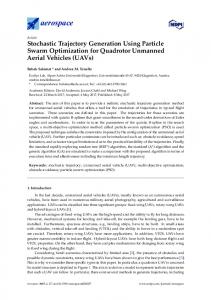
The comparison of the obtained runtimes is shown in Table II. The success rate remained the same, thus we do not show it. For both “Easy” and “Hard” unconstrained tests, the runtime grew by approximately 30%. For the test with orientation constraints, the runtime growth reached 71% which is explained by many disjoint local minima caused by the constraints, which is harder to overcome. However, the full cost function allowed to obtain trajectories with lower durations and torques. We demonstrate the effects of these components in the next subsections. Overall, the runtime growth is not critical. Our method may be used in a frequentreplanning manner for acting in dynamic environments. 2) Obstacle costs: In this experiment, we demonstrate how different obstacle cost component importance weights influence the obtained solutions. We took a task from the shelf experiment and obtained solutions with three different obstacle importance weights, shown in Fig. 5. While the trajectory with the value of obstacle cost weight 1.0 is the safest, as it moves the arm very far from the obstacles, this trajectory is the longest and has the longest duration. The trajectory with lowest obstacle weight is the fastest to execute, but includes movements close to the obstacles. 3) Torque optimization: In order to demonstrate how torque optimization influences the resulting trajectory, we performed an additional experiment. The initial configuration is a default position of the robot with bent elbow. The goal configuration has fully extended arm and the torso is rotated. The weight of the end-effector is being increased by 5 kg representing a heavy object in the hand. The optimization is performed two times: with and without torque minimization. The obtained trajectories are depicted in Fig. 6. Without torque minimization, all joints move uniformly towards the goal. With torque minimization turned on, the trajectory is different. The arm in the extended state experiences high torques due to gravity. The optimizer avoids this effect by keeping the arm bent and rotating the torso first. Only when this movement is finished, the arm is extended, which results in lower total torque. 4) Duration optimization: In this experiment, we demonstrate the behaviour of our duration cost component. We took a task from the shelf experiment and adjusted the goal configuration in a way that it is located very close to the cell border, so that in the end the robot must move close

(a)

(b)

(a) Trajectory with both start and goal velocities 0 rad/s.

(b) Velocity vs time for (a).

(c) Trajectory with start velocity 0.7 rad/s and goal velocity 0 rad/s.

(d) Velocity vs time for (c).

Fig. 6. Comparison of trajectories obtained with/without torque optimization. The robot is assumed to hold 5 kg. Red: without torque optimization; Green: with torque optimization. (a) Trajectories of the end-effector. Black: start pose; Yellow: goal pose. With torque optimization the robot first rotates the torso and only then extends the arm, which results in lower torque. (b) Magnitude of the total torque. Without optimization (upper line) the torque grows faster and reaches unnecessary high values. While with optimization (lower line) total torque grows slower.

(a)

(b)

Fig. 8. Example of a duration optimization. Black: start pose; Yellow: goal pose. The grey-scale lines represent the trajectories of the end-effector. The brighter the segment is, the larger is the velocity. In the first case (a) the initial and the goal velocities are 0 rad/s. In the second case (c) the initial velocity is 0.7 rad/s. In both cases the optimizer attempts to reach the maximum velocity and keeps it as long as possible before deceleration. However, as in (c) the velocity is non-zero initially, there is less time spent for acceleration, and hence, the overall duration is smaller.

Fig. 7. Duration optimization. In order to make the movement safer, the optimizer maintains lower velocities in region near the obstacles. This makes an earlier deceleration necessary, which results in a trajectory with longer duration, but with a higher safety level. (a) The grey-scale line represents the trajectory of the end-effector. The brighter the segment is, the larger is the velocity during that segment. Black: start pose; Yellow: goal pose. (b) Velocity vs time.

to the obstacle. The obtained solution is shown in Fig. 7 As the movement starts and ends in a static state, both initial and goal velocities were set to 0 rad/s. One can see that the algorithm attempts to reach the maximum allowed velocity (1.0 rad/s) during the first part of the trajectory and then maintains this velocity. However, as further movement is done close to the obstacle, the deceleration is started in advance and the movement is continued towards the goal with low velocity, which makes the motion safer. To demonstrate replanning capabilities of our method, we performed an additional experiment. The optimization is done two times: in the first case start and goal velocities are 0 rad/s. In the second case, the initial velocity is 0.7 rad/s and the goal velocity is 0 rad/s. The experiment shows that our method can be used for replanning when the robot is already moving. Resulting trajectories are shown in Fig. 8. One can observe that in both cases the velocity smoothly grows towards its maximum allowed value (1.0 rad/s). It stays on this level and then decreases until the goal value is reached. The trajectory which starts with 0.7 rad/s velocity has smaller duration (2.78 s) than the trajectory which starts with 0 rad/s (3.81 s), which is an expected result.

(a)

(b)

Fig. 9. Obstacle avoidance with a real robot. (a) Planned trajectory which avoids the obstacle in order to reach a pre-grasp pose. (b) Momaro executing the planned trajectory.

B. Robot Experiments To demonstrate that our method can be applied in reality, experiments with real robots were performed. The videos of the experiments are available online3 . 1) Momaro: We used our method to reach a pre-grasp pose with the Momaro robot. As shown in Fig. 9, Momaro successfully avoided an obstacle placed on the way. This demonstration was shown live during the review meeting of the CENTAURO4 project. Different obstacle cost importance weights were used to avoid the obstacle with different margins, to demonstrate planning of safe or fast trajectories. 3 http://www.ais.uni-bonn.de/videos/IROS_2017_ Trajectory_Optimization 4 https://www.centauro-project.eu

R EFERENCES [1] [2]

[3] [4] (a)

(b)

Fig. 10. Replanning with iiwa arm. (a) Two trajectories: initial (lower line) and replanned (upper line), which was produced when previously unconsidered obstacle (box in the middle) interfered the initial trajectory. (b) iiwa arm executing a replanned trajectory, avoiding the previously unconsidered obstacle (box).

[5] [6]

[7]

2) KUKA arm: STOMP-New was used during the Showcase evaluation of the KittingBot project in the European Robotics Challenge 2 (EuRoC)5 . In this challenge, the KUKA miiwa robot was used, which consists of an iiwa manipulator on an omnidirectional mobile base. The objective was to pick up different engine parts in different locations across the arena. Our method was used to plan trajectories for the iiwa arm to reach a pre-grasp pose and to deliver a grasped object to a pre-release pose. There were three different objects: metal engine support parts of two sizes and engine pipes. In order to plan trajectories with these objects during one run, rough approximations of these objects were attached and detached from our collision model. In addition, we performed a replanning experiment, which shows the capability of our method to perform a quick replanning when an obstacle interferes with the already planned trajectory. In Fig. 10 one can see the robot executing the final trajectory, replanned to avoid the box. V. C ONCLUSIONS In this paper, we presented an approach for optimization of arm trajectories with respect to multiple criteria that extends STOMP. Trajectory duration is optimized by including a velocity into the configuration space. We proposed a multicomponent cost function, which includes the following cost components: collisions, joint limits, orientation constraints, joint torque and trajectory duration. The components are normalized and have importance weights assigned. These weights allow to prioritize component optimization and obtain trajectories with different properties. The cost function is designed to evaluate a trajectory efficiently, keeping the computational load as low as possible. It is easy to extend the cost function with any additional costs as long as they are normalized. We evaluated our method in simulation and on real robots. Our approach demonstrated high success rate and low runtime, making it suitable for frequent replanning in dynamic environments.

[8]

[9]

[10] [11]

[12]

[13] [14] [15]

[16] [17] [18] [19]

[20]

[21] [22]

5 http://www.euroc-project.eu/index.php

M. Kalakrishnan, S. Chitta, E. Theodorou, P. Pastor, and S. Schaal, “STOMP: Stochastic trajectory optimization for motion planning”, in IEEE Int. Conf. on Robotics and Automation (ICRA), 2011. R. B. Rusu, I. A. Sucan, B. Gerkey, S. Chitta, M. Beetz, and L. E. Kavraki, “Real-time perception-guided motion planning for a personal robot”, in IEEE/RSJ Int. Conf. on Intelligent Robots and Systems (IROS), 2009, pp. 4245–4252. R. Diankov, N. Ratliff, D. Ferguson, S. Srinivasa, and J. Kuffner, “BiSpace planning: Concurrent multi-space exploration”, in Robotics: Science and Systems (RSS), 2008. S. M. Lavalle, “Rapidly-exploring random trees: A new tool for path planning”, Tech. Rep., 1998. J. James J. Kuffner and M. Steven, “RRT-Connect: An efficient approach to single-query path planning”, in IEEE Int. Conf. on Robotics and Automation (ICRA), 2000, pp. 995–1001. J. D. Gammell, S. S. Srinivasa, and T. D. Barfoot, “Informed RRT*: Optimal sampling-based path planning focused via direct sampling of an admissible ellipsoidal heuristic”, in IEEE/RSJ Int. Conf. on Intelligent Robots and Systems (IROS), 2014, pp. 2997–3004. J. D. Gammell, S. S. Srinivasa, and T. D. Barfoot, “Batch Informed Trees (BIT*): Sampling-based optimal planning via the heuristically guided search of implicit random geometric graphs.”, in IEEE Int. Conf. on Robotics and Automation (ICRA), 2015, pp. 3067–3074. L. Janson and M. Pavone, “Fast Marching Trees: A fast marching sampling-based method for optimal motion planning in many dimensions”, in Robotics Research: The 16th International Symposium (ISRR). 2016, pp. 667–684. F. Burget, M. Bennewitz, and W. Burgard, “BI2RRT*: An efficient sampling-based path planning framework for task-constrained mobile manipulation”, in IEEE/RSJ Int. Conf. on Intelligent Robots and Systems (IROS), 2016, pp. 3714–3721. M. Stilman, “Global manipulation planning in robot joint space with task constraints”, IEEE Transactions on Robotics, vol. 26, no. 3, pp. 576–584, 2010. A. Perez, S. Karaman, A. Shkolnik, E. Frazzoli, S. Teller, and M. R. Walter, “Asymptotically-optimal path planning for manipulation using incremental sampling-based algorithms”, in IEEE/RSJ Int. Conf. on Intelligent Robots and Systems (IROS), 2011. T. Kunz and M. Stilman, “Probabilistically complete kinodynamic planning for robot manipulators with acceleration limits”, in IEEE/RSJ Int. Conf. on Intelligent Robots and Systems (IROS), 2014, pp. 3713–3719. N. Ratliff, M. Zucker, J. A. D. Bagnell, and S. Srinivasa, “CHOMP: Gradient optimization techniques for efficient motion planning”, in IEEE Int. Conf. on Robotics and Automation (ICRA), 2009. O. Brock and O. Khatib, “Elastic Strips: A framework for motion generation in human environments”, The International Journal of Robotics Research, vol. 21, no. 12, pp. 1031–1052, 2002. A. Byravan, B. Boots, S. Srinivasa, and D. Fox, “Space-Time functional gradient optimization for motion planning”, in Proceedings - IEEE Int. Conf. on Robotics and Automation (ICRA). 2014, pp. 6499–6506. R. Steffens, M. Nieuwenhuisen, and S. Behnke, “Continuous motion planning for service robots with multiresolution in time”, in 13th Int. Conf. on Intelligent Autonomous Systems (IAS). 2016, pp. 203–215. Q.-Z Ye, “The signed Euclidean distance transform and its applications”, 9th Int. Conf. on Pattern Recognition (ICPR), 1988. M. L. Felis, “RBDL: An efficient rigid-body dynamics library using recursive algorithms”, Autonomous Robots, pp. 1–17, 2016. M. Schwarz, T. Rodehutskors, D. Droeschel, M. Beul, M. Schreiber, N. Araslanov, I. Ivanov, C. Lenz, J. Razlaw, S. Sch¨uller, D. Schwarz, A. Topalidou-Kyniazopoulou, and S. Behnke, “NimbRo Rescue: Solving disaster-response tasks through mobile manipulation robot Momaro”, Journal of Field Robotics, 2016. I. A. S¸ucan and L. E. Kavraki, “Kinodynamic motion planning by interior-exterior cell exploration”, in Algorithmic Foundation of Robotics VIII: Selected Contributions of the Eight Int. Workshop on the Algorithmic Foundations of Robotics. 2010, pp. 449–464. R. Bohlin and L. E. Kavraki, “Path planning using lazy PRM”, in Int. Conf. on Robotics and Automation (ICRA), 2000, pp. 521–528. I. A. S¸ucan, M. Moll, and L. E. Kavraki, “The Open Motion Planning Library”, IEEE Robotics & Automation Magazine, pp. 72–82, 2012.