Electrical Load Forecasting in Power Distribution

International Journal of Electronics Communication and Computer Engineering Volume 4, Issue 6, ISSN (Online): 2249–071X, ISSN (Print): 2278–4209

Electrical Load Forecasting in Power Distribution Network by Using Artificial Neural Network Ali Nahari

Habib Rostami*

Rahman Dashti

Electrical Engineering Department, School of Engineering, Persian Gulf University of Bushehr, Bushehr 75168, Iran. Email: [email protected]

Computer Engineering Department, School of Engineering, Persian Gulf University of Bushehr, Bushehr 75168, Iran. Email: [email protected]

Electrical Engineering Department, School of Engineering, Persian Gulf University of Bushehr, Bushehr 75168, Iran. [email protected]

Abstract – Today, one of most important concerns in electrical power markets and distribution network is supplying the customer demands. In order to manage the market it is necessary to forecast the usage of electrical power in distribution network. The pattern of electrical power usage depends on many different parameters such as the week days, seasons, weather condition and etc. Today, researchers by using an artificial intelligence based on the natural intelligence are trying to forecast the costumers’ usage of electrical power. In this Paper it is tried to forecast the electrical power usage according to weather data by using artificial neural network in Bushehr distribution electrical power network and also is tried to find out the pattern of electrical power usage with the dataset which is prepared by real data. The method which has been used here is useful in all kind of power forecasting such as short term, middle term and long term. It can be helpful to manage the distributed generators production schedule and also correction of electrical power usage. Keywords – Artificial Neural Network, Back Propagation, Distribution Network, Electrical Power, Load Forecasting.

I. INTRODUCTION

includes temperature, humidity, and atmospheric pressure historical data in Libya and classified weather data as input before training which would cause to increase the processing terms and also in this paper did not attention to time of power consumption while that is an important factor in power consumption.Reference [3] used weather data as the input which contains max and min of temperatures, humidity for short term load forecasting in India. In reference [4] Multi-layer Perceptions network is used to estimate the load in short term by using 2 variables; the historical load demand and time. The author of reference [5] used the ANN to forecast electrical power load according to hours in short term. In reference [6] the ANN is used to short term forecast load according to hours, the day of the week and weather data which is made simple as seasons’ values. Reference [7]contributes to a practical method for short-term load forecasting, especially as it shows the effect of seasonal variation on load curve forecasting.In this paper is tried to find out the way to forecast the electrical power load in Bushehr power distribution network by using artificial neural network with the help of Matlab software. The input is involved 4 feature; time, temperature, wind speed and humidity. This parameters effect on power consumption directly. Mean square error is used as performance measure. The method of learning in ANN which is used in this paper is back propagation. Finally by comparing different cases is tried to find best solution to estimate the load of 20Kv/400v substation.

Electrical power distribution companies have to manage distribution network which is one of the most important parts of the power system. Some parameters such as reliability, power loss, voltage profile and etc are more important in this part of power system and this is all because of being the large number of customer in distribution networks. It is necessary to forecast the electrical load to generate power in network. Some II. ANN parameters effect on load profile. These parameters can be different like weather condition, work days and holydays, Load estimating is done in two ways: seasons, price of each Kwh, kind of customers such as A. Statistical methods: forecasting the load is based on residential, industrial and commercial and some others. statistical data processing in this method. These parameters can be used in forecasting the electrical B. Modern methods: in this method Artificial load which is classified in four classes:  Very Short term load forecasting: The load forecasting Intelligence techniques are used. Modern load forecasting techniques, such as expert systems, artificial neural for 1 minute to few hours.  Short term load forecasting: The load forecasting for 1 networks (ANN), fuzzy logic, wavelets, have been developed recently, showing encouraging results. Among day to 1 week.  Medium term load forecasting: The load forecasting them, ANN methods are particularly attractive, as they have the ability to handle the nonlinear relationships from several weeks to one or several years.  Long term load forecasting: The load forecasting up to between load and the factors affecting it directly from historical data [8]. In this paper, we use back propagation 20 years. Base on the condition and necessity one of these classes feed-forward neural network to model the problem. Each is used in load forecasting. Reference [1] introduces a neural network has at least three layers, input layer, a brief overview in long term forecasting methods. In hidden layer and output layer. In a typical Multilayer reference [2] the author used the ANN to learn the network, the input units which are denoted by Xi are relationship between daily load and weather condition that connected to all hidden layer units which are defined by Yj Copyright © 2013 IJECCE, All right reserved 1737

International Journal of Electronics Communication and Computer Engineering Volume 4, Issue 6, ISSN (Online): 2249–071X, ISSN (Print): 2278–4209 and the hidden layer units are connected to all output layer units which are denoted by Zk. The elements Wij or Vij of the weight matrix associate the weight of each connection between the input to hidden and hidden to output layer units. The hidden and output layer units also receive signals from weighted connections (bias) from units whose values are always 1.

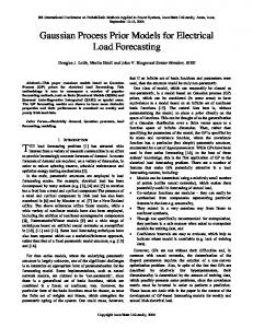
Bushehr province is about 25360 Km2 and a city with same name is its capital. Bushehr is in the south of Iran and its geographic position is between 27', 14'' to 30', 16'' north latitude and 50', 6 '' to 52', 58'' east longitude.[9] Bushehr is a port with tropical climate that cause to increase of power consumption. In the other hand it can be said that its climate has most effect on the load pattern. Fig 3 shows the changes of weather and the load profile in 3rd of December of 2010.

Fig.2. Geographical position of Bushehr Fig1.Neural Network In each output and hidden units the incoming signals from the previous layer sums together and apply an activation function to form the response of the net for a given input pattern. .X i  input [i ]. (1)

X W  Y V

.Y j  f ( b j 

i

ij

).

(2)

(3) .Z k  f ( bk j jk ). To determine the error each output will be compare its output (Zk) with the actual output value which is identified by dk. Then according to the calculated error, 𝞭k will be determined.  k is a factor which is used to distribute the error at Zk back to all units in the previous layer. (4) . k = f (Zk )(d k - Zk ). Factor  j will be computes for each hidden unit. This

(a)

factor is a weighted sum of all the back propagated delta terms from units in the previous layer multiplied by the derivative of the activation function for that unit. (5) . j = f (Yj )  k Vjk . In the next step the new value of bias and each element of weight matrix will be calculated where η is a learning rate coefficient that is given a value between 0 and 1 at the start of training. (6) .b j (new) = b j (old) +  j . .Wij (new) = Wij (old) +  j X i .

(7)

(b)

In each irritation it will be checked if the stop condition is occurred or not. The stop condition can be reaching error threshold, defined irritation and etc.

III. DATASET The dataset is 533 samples of four elements so the dataset is the matrix that has 533 rows and five columns which its 1st column is time, the 2nd column is air temperature, the 3rd one is humidity, 4th one is wind speed and the last column is customers' electrical power usage. This dataset is about the weather of Bushehr and its electrical power distribution network. Copyright © 2013 IJECCE, All right reserved 1738

\ (c)

International Journal of Electronics Communication and Computer Engineering Volume 4, Issue 6, ISSN (Online): 2249–071X, ISSN (Print): 2278–4209

IV. SIMULATION

600000 500000

Watt

400000 300000 200000 100000

0:00 2:00 4:00 6:00 8:00 10:00 12:00 14:00 16:00 18:00 20:00 22:00

0

Time

(d) Fig 3.The weather changes and the load profile in 24 Hours. (a) Air Temperature in Centigrade (b) Relative humidity in percentage (c) Wind Speed in meter per second (d) Electrical power load profile in Watt.

In this paper is tried to find the way to forecast the Power Usage. The method that is used is ANN and the Levenberg-Marquardt Back-propagation is the algorithm which is used to learn the network. The network setting is original back propagation 4 inputs and 1 output. The hidden layers, the learning rate setting, momentum and number of Epoch changes in the cases while stopping criteria is 0.008 and the performance measure is MSE (Mean Square Error). The weather Information is taken from reference [10]. And the Information about the electrical power usage is taken from Bushehr Distribution Company. The period of study is for eight month from May 2008 till December 2008. In Some Cases the Dataset is inserted as their real Value and in some others is normalized. The information about different cases is described in the following table.(n) Shows that the Dataset has been normalized and T shows that tansin is used as function and also P is the sign of using purelin and logsig is shown by L.

Table I: Information of study on different cases Num of Inputs Case (1)

4

Case (2)

4 (n)

Case (3)

4

Case (4)

4 (n)

Case (5)

4 (n)

Case (6)

4 (n)

Case (7)

4 (n)

Case (8)

4 (n)

Case (9)

4 (n)

Case (10)

4 (n)

Case (11)

4 (n)

Case (12)

4 (n)

Case (13)

4 (n)

Case (14)

4 (n)

Case (15)

4 (n)

Case (16)

4 (n)

Num of nodes in hidden layers 3 P 3 L 6 P 6 T 3 T 6 T 6 T 10 T 10 T 10 T 15 T 20 T 20 T 20 T 20 T 20 T

2 P 2 L 2 P 2 T 2 T 3 T 4 T 3 T 3 T 6 T 6 T 6 T 10 T 15 T 15 T 15 T

1 P 1 L 1 P 1 T 1 P 2 T 2 T 2 T 2 T 4 T 4 T 3 T 5 T 10 T 10 T 10 T

1 P 1 T 1 T 1 T 2 T 2 T 1 T 1 T 5 T 5 T 5 T

1 T 1 T

1 T 1 T 1 T

Num of epoch

Learning Rate

Goal

MC

2000

0.015

0.008

0.95

20000

0.015

0.008

0.95

20000

0.015

0.008

0.95

20000

0.015

0.008

0.95

20000

0.015

0.008

0.95

20000

0.015

0.008

0.95

20000

0.015

0.008

0.95

20000

0.015

0.008

0.95

20000

0.020

0.008

0.85

20000

0.015

0.008

0.95

20000

0.015

0.008

0.95

20000

0.015

0.008

0.95

20000

0.015

0.008

0.95

20000

0.015

0.008

0.95

20000

0.020

0.008

0.85

20000

0.010

0.008

0.98

Copyright © 2013 IJECCE, All right reserved 1739

International Journal of Electronics Communication and Computer Engineering Volume 4, Issue 6, ISSN (Online): 2249–071X, ISSN (Print): 2278–4209

V. RESULT OF SIMULATIONS The result of simulations is presented in the following table and Fig 4 to 19.

Fig.7. Regression plot of study on case 4

Fig.4. Regression plot of study on Case 1

Fig.8. Regression plot of study on Case 5

Fig.5. Regression plot of study on case 2

Fig.9. Regression plot of study on Case 6

Fig.6. Regression plot of study on case 3

Fig.10. Regression plot of study on Case 7 Copyright © 2013 IJECCE, All right reserved 1740

International Journal of Electronics Communication and Computer Engineering Volume 4, Issue 6, ISSN (Online): 2249–071X, ISSN (Print): 2278–4209

Fig.11. Regression plot of study on Case 8

Fig.15. Regression plot of study on Case 12

Fig.12. Regression plot of study on Case 9

Fig.16. Regression plot of study on Case 13

Fig.13. Regression plot of study on Case 10

Fig.17. Regression plot of study on Case 14

Fig.18. Regression plot of study on Case 15 Fig.14. Regression plot of study on Case 11 Copyright © 2013 IJECCE, All right reserved 1741

International Journal of Electronics Communication and Computer Engineering Volume 4, Issue 6, ISSN (Online): 2249–071X, ISSN (Print): 2278–4209

Fig.19. Regression plot of study on Case 16 Fig 7 to 19 shows the regression plot. The regression plot has 2 axes; the vertical axis is output of training and horizontal axis. In the regression plot the target values and the output values are located as pairs in the coordinate

Case (1) Case (2) Case (3) Case (4) Case (5) Case (6) Case (7) Case (8) Case (9) Case (10) Case (11) Case (12) Case (13) Case (14) Case (15) Case (16)

plot. If both of them be the same they will be located on the diameter of the square plot and if the point be far from the diameter that means the output is differ from target. It can be said if the point be more far from diameter more difference is reached.In the regression, whatever the blue line is closer to the diameter shows the better and more accurate results. The R which is written in the top of the plot is r-square error and whatever its value b closer to 1 is better. As the result shows, by increasing the hidden layers and the nodes the better performance goal will be reach in the lowest iterations. The last six cases’ regression plots prove this matter. In these cases the r-square error is more than 0.98 and the case 15 is the best one with the r-square error equal to 0.98573. In the last 6 cases by meeting the performance goal the training has been stopped. By increasing the hidden layers the iteration decreases. And also by analyzing the results of cases 1 to 5 it can be figure out that normalized input data has better results than unnormalized ones.

Table II: Result of Training in different cases Num Of Iterations Performance Gradient MU 13 2.89*109 7.38*10-5 1*1011 2611 0.184 9.98*10-6 0.01 9 23 2.89*10 3.02*10-5 1*1011 6147 0.0239 9.87*10-6 1*10-8 -5 20000 0.0219 5.02*10 1 -6 658 0.0242 9.60*10 0.01 20000 0.0189 0.000648 0.1 666 0.0140 9.77*10-6 0.01 602 0.0171 9.94*10-6 0.1 20000 0.0107 0.000240 0.1 189 0.00799 0.00174 0.01 71 0.00792 0.00727 0.001 69 0.008 0.00117 0.01 54 0.00795 0.115 0.01 28 0.00764 0.0546 0.01 30 0.00771 0.0482 0.01

VI. CONCLUSION

The Reason of Stopping Max Mu reached Min gradient reached Max Mu reached Min gradient reached Max epoch reached Min gradient reached Max epoch reached Min gradient reached Min gradient reached Max epoch reached Performance goal met Performance goal met Performance goal met Performance goal met Performance goal met Performance goal met

REFERENCES

L. Ghods and M. Kalantar, “Different Methods of Long-Term The result of this research shows the high efficiency of [1] Electric Load Demand Forecasting; A Comprehensive Review” the neural network in estimating the electrical power load. Iranian Journal of Electrical & Electronic Engineering, vol. 7, All this because the ANN can define the nonlinear relation No. 4, Dec. 2011, pp. 249–259. between the weather data and the load with high [2] Ammar. K. Mahmoud, “Information system for forecasting processes based on unsupervised, supervised neural networks” Accuracy. And also it can be said that this method is not International Journal of Computer Science & Engineering limited to any of the classes that described before because Technology (IJCSET), vol. 4, No. 2, Feb. 2013, pp. 162–172. if we have the weather parameters it is possible to forecast [3] K. Geetha andSk.Mohiddin, “Short Term Load Forecasting using the load. By using ANN for forecasting the long term Generalized Neuron Model with Error Gradient Functions” International Journal of Advanced Research in Computer weather situation, the method which is presented in this Science and Software Engineering, vol. 3, Issue 4, April 2013, paper can be used for long term load forecasting. This pp. 357–360. research and generally every research about load [4] SamsherKadir Sheikh and M. G. Unde, “Short-Term Load forecasting can be helpful for scheduling on requirement Forecasting using ANN Technique” International Journal of Engineering Sciences & Emerging Technologies, vol. 1, Issue 2, on developing electrical distribution network, switching, Feb 2012, pp. 97–107. selling energy, maintenance and repairment and also standing by the DG sources. Copyright © 2013 IJECCE, All right reserved 1742

International Journal of Electronics Communication and Computer Engineering Volume 4, Issue 6, ISSN (Online): 2249–071X, ISSN (Print): 2278–4209 [5]

[6]

[7]

[8]

[9]

[10]

Muhammad Buhari, and SanusiSaniAdamu, “Short-Term Load Forecasting Using Artificial Neural Network” Proceeding of the International MultiConerence of Engineers and Scientists, vol. 1, Mar 2012. M. Sarlak, T. Ebrahimi and S. S. KarimiMadahi, “Enhancement the accuracy of daily and hourly Short Time Load Forecasting using Neural Network” Journal of Basic and Applied Scientific Research, 2012, pp. 247–255. By ParasMandal, TomonobuSenjyu, Naomitsu Urasaki and Toshihisa Funabashi, “A neural network based several-hourahead electric load forecasting using similar days approach” Electrical Power and Energy Systems 28, 2006, pp. 367–373. BadarUl Islam, “Comparison of Conventional and Modern Load Forecasting Techniques Based on Artificial Intelligence and Expert Systems” IJCSI International Journal of Computer Science Issues, vol. 8, No. 3, Sep 2011, pp. 504–513. A. Nahari and R. Dashti, “Technical and economic analysis of different micropowers in providing network load and optimal selection with real load analysis of a 20KV/400V station in Bushehr Province of Iran.” Advanced Power System Automation and Protection, 2011. http://www.wunderground.com

AUTHOR’S PROFILE Ali Nahari was born in Bushehr, Iran, on Sep 16, 1985. He received the B.Sc. in electrical power engineering in 2008. He is currently pursuing a M.Sc. degree in electrical power engineering. His research interests are distribution system and DG especially in Photovoltaic system, cathodic protection systems.

Habib Rostami received B.Sc., M.Sc. and Ph.D in computer Engineering from Sharif University of Technology, Iran. Now he is an assistant professor in Persian Gulf University, Bushehr, Iran. His interest includes network analysis, Data mining, Pattern Recognition and Graph Theory.

Rahman Dashti was born in Bushehr, Iran, on Sep 22, 1982. He received the B.Sc. in electrical engineering from Shiraz University in 2004 and the M.Sc. from Iran University Science and Technology in 2006 and the Ph.D from Ferdowsi University of Mashhad, Iran in 2013. Since then he served as an assistant professor at the Persian Gulf University of Bushehr. His research interests are Power System Protection, Electromagnetic Transients in Power System, distribution system, protection and control technique to distribution system, DG.

Copyright © 2013 IJECCE, All right reserved 1743