Si Gwan Kim. Dept. of Computer .... In [18], the minimum distance tree (MD-tree) is separately ..... [9] F. Ye, H. Luo, J. Cheng, S. Lu, L. Zhang, "A Two-tier data.
(IJACSA) International Journal of Advanced Computer Science and Applications, Vol. 3, No.2, 2012
Energy-Efficient Dynamic Query Routing Tree Algorithm for Wireless Sensor Networks Si Gwan Kim
Hyong Soon Park
Dept. of Computer Software Kumoh Nat’l Inst. of Technology Gumi, Korea
Gumi Electronics & Information Technology Research Gumi, Korea
Abstract— To exploit in answering queries generated by the sink for the sensor networks, we propose an efficient routing protocol called energy-efficient dynamic routing tree (EDRT) algorithm. The idea of EDRT is to maximize in-network processing opportunities using the parent nodes and sibling nodes. Innetwork processing reduces the number of message transmission by partially aggregating results of an aggregate query in intermediate nodes, or merging the results in one message. This results in reduction of communication cost. Our experimental results based on simulations prove that our proposed method can reduce message transmissions more than query specific routing tree (QSRT) and flooding-based routing tree (FRT). Keywords- sensor networks; routing trees; query processing.
I. INTRODUCTION Wireless sensor networks have emerged as an innovative class of networked systems due to the union of smaller, cheaper embedded processors and wireless interfaces with sensors based on micro-mechanical systems (MEMS) technology. Each node is equipped with one or more sensors, storage and processing resources, and communication subsystems. Each sensor is specialized to monitor a specific environmental parameter such as thermal, optic, acoustic, seismic, or acceleration. The nodes are distributed in the sensing phenomenon. Typical sensor networks incorporate into a variety of military, medical, environmental, and commercial applications. Sensor networks often contain one or more sinks that provide centralized control. A sink typically serves as the access point for the user or as a gateway to another network. Large sensor networks can be composed of thousands of sensor nodes deployed in the field to observe a region. Sensor networks have several major constraints: limited processing power, limited storage capacity, limited bandwidth, and limited energy. Researchers are working to solve many of the limitations affecting sensor nodes and networks. Some researchers are working to improve node design; others are developing improved protocols associated with a sensor network; still others are working to resolve security issues. Energy efficiency has been a major concern in sensor networks because most sensor nodes have limited power. If used without care, they will deplete their power quickly [1][2][3][4]. It is known that message communication among sensor nodes is a main source of energy consumption. Typically, wireless communication consumes several thousand
times more energy than computation [5]. In the tree-based approach [6][7] a spanning tree rooted at the sink is constructed first. Subsequently this tree is exploited in answering queries generated by the sink. This is done by performing in-network aggregation along the aggregation tree by proceeding level by level from its leaves to its root. The main idea of in-network processing is to reduce volumes of data in the network by partially aggregating sensed values or merging intermediate data. For aggregation queries such as MAX, SUM and COUNT, an intermediate node may aggregate them and send only a newly computed value instead of just forwarding all values received from its children. For example, for a SUM query, an intermediate node forwards only the added value among the values received from its children. These aggregate queries reduce the number of messages, thus reducing power consumption. In this paper, we propose a query-based routing tree, called energy-efficient dynamic routing tree (EDRT) that is separately constructed for each query by utilizing the query information. The main objective of the EDRT is to minimize the number of hops by increasing the amount of data merge processing, thus reducing the total number of generated messages to reach the destination. The EDRT is constructed in such a way that messages generated from sensor nodes can be merged more often and earlier. This paper is organized as follows. Section 2 discusses the related works; Section 3 formally defines the EDRT and describes how to construct EDRT in sensor networks. Experimental evaluation of EDRT is presented in Section 4. Finally Section 5 concludes the paper. II.
RELATED WORKS
There has been a lot of work on query processing in distributed database systems, but major differences exist between sensor networks and traditional distributed database systems[8][9][10][11][12]. As sensor networks have limited capabilities such as energy consumption and computation, query processing in sensor networks must take into account these constraints. Much work in construction of efficient routing trees in sensor networks has been done in sensor network applications [13][14][15][16]. When centralized querying is employed in WSN, the base station acts as the point where the query is introduced and results are gathered. The TinyDB Project at Berkeley [17], which is largely used for data gathering in sensor networks,
123 | P a g e www.ijacsa.thesai.org
(IJACSA) International Journal of Advanced Computer Science and Applications, Vol. 3, No.2, 2012
uses spanning trees for the data retrieval, but does not rely on any other in-network data to optimize queries. This centralized technique may not be feasible for self-organizing sensor networks since a query may be initiated from any node in the network and propagating the query to the base station would cost too much. A semantic routing tree (SRT) is a routing tree used in query dissemination to route a query to the nodes that have a possibility to generate tuples for the query. By sending a query only to the nodes that need to receive the query, the SRT can reduce communication cost in query dissemination. In [18], the minimum distance tree (MD-tree) is separately constructed for each query by utilizing the query information. The MD-tree can increase the amount of in-network processing by constructing the tree in such a way that messages generated from sensor nodes can be merged more often and earlier, thus minimizing the energy consumption. In [19], a query routing trees are formed by balancing the data load to be transmitted from one tree level to the next. The goal is to balance the data received and relayed by each node in the network. The energy savings in this tree are mostly theoretical since they do not deal with collisions occurring from many nodes trying to communicate with the same parent. Reference [20] proposes the design of a distributed index that scalably supports multi-dimensional range queries. Distributed index for multi-dimensional data (or DIM) uses a novel geographic embedding of a classical index data structure, and is built upon the GPSR geographic routing algorithm. DIFS [21] extends traditional binary-tree and quad-tree by allowing multiple parents and multiple roots. In DIFS, a node may have several parents, which may be located far away. This leads to distance sensitivity problem. Thus constructing the DIFS tree and update operations are expensive. But DIFS scales well to large-scale networks by using a multiply rooted tree and a geography/value coverage tradeoff that balances communication overhead over many nodes. III. ENERGY-EFFICIENT DYNAMIC ROUTING TREE In this section, we present our energy efficient routing algorithm based on dynamic routing tree. A. Definition We model a sensor network as an undirected graph G = (V, E) where V is a set of nodes and E is a set of edges. A root node can be act as a base station. An edge (vi,vj) is in E if two nodes vi and vj can communicate each other. Fig. 1 shows a graph for a sensor network with 8 nodes. The distance from vi to vj in graph G for a sensor network is defined to be the length of a path from vi to vj with the minimum number of edges. The distance from the root node to vi is called the “distance of vi” . In Fig. 1, v1 is a root node and distance of v7 is 3. Parent candidate set CPi and sibling candidate set CSi for sensor node i is defined as follows. CPi = { vi | vj is a neighbor of vi and lj = li - 1} CSi = { vi | vj is a neighbor of vi and lj = li}
Figure 1. Example of a sensor network
In other words, parent candidate set CPi is a set of neighbour node that is lower level by one than the given node i. And sibling candidate set CSi is a set of neighbour node that is same level with the given node i. A query node is a node which satisfies the query qualification conditions in the WHERE clause of the query. For convenience, the root node is considered as a query node for every query regardless of satisfying the qualification of the query. The minimum distance of node i for query Q, denoted by MDi,Q is defined as follows: {
{
}
In other words, if sensor node i is a root node or a candidate node for a query, is 0. Otherwise, is added by 1 the smallest value of the parent candidate set. We use the term md instead of MDi,Q for brevity if node i for query Q is known in advance. Candidate parent md set for node i is defined to be a collection of MDi,Q for CPi. Each member of this set consists of node id and md value. Candidate sibling md set for node i is a collection of MDi,Q for CSi. Each member of this set consists of node id and md value as in . But, if md value is not 0, md – 1 is stored. The first node to be received for query Q, denoted as Pi,Q, is a node which has the smallest md value among candidate parent and candidate sibling set. In other words, Pi,Q = MinDistId ( ), where MinDistId is a function which returns the id of the smallest md value. If there is more than one node which has the smallest value, the smaller level is selected, and if levels are same, random node is selected. B. Our Algorithm In this section, we present the process of our algorithm. This process consists of two stages.
Candidate Set Decision Stage: This stage determines the parent candidate set and sibling candidate set for each node.
Query Dissemination and EDRT Construction Stage: When a user requests a query, the EDRT for the query is constructed through the query dissemination. Each sensor node calculates the md value and sends the
124 | P a g e www.ijacsa.thesai.org
(IJACSA) International Journal of Advanced Computer Science and Applications, Vol. 3, No.2, 2012
query message with this value to neighbor nodes which has the smallest md value. 1) Candidate Set Decision Stage In this stage, parent and sibling candidate sets are determined for each node. Candidate decision message, denoted as CDM, includes dest_id, src_id and level, where dest_id is the destination node identifier, src_id is the sender node identifier and level is the level of sender node. The level of root node is 0. In Fig. 2, the path taken by the candidate decision messages are shown in arrows and candidate sets CPi and CSi are shown. In Fig. 3, candidate decision processes are shown.
Input: CDM (dest_id / src_id / level), Node i with leveli = INVALID_VALUE, CPi = and CSi = Output: Node i with level , CPi , CSi Step : 1. Sink node transmits candidate decision message to root node. 2. Root node broadcasts the message with its identifier value src_id and its level. 3. When a node receives the message, it checks the following case. if (level of node i == INVALID_VALUE) { Set level of node i as value of level field in CDM plus 1 Add src_id to CPi Broadcast the message with its identifier and level } else { if (level field in CDM == (level of node i) - 1 ) { Add src_id to CPi } else if (level field in CDM == (level of node i) ) { Add src_id to CSi } } 4. This process is repeated until all the nodes in the network decide their levels, parent and sibling candidate sets. Figure 3. Candidate Decision Processes
Figure 2. Example of Candidate Set Decision
2) Query Dissemination and EDRT Construction Stage When a user requests a query, the EDRT for the query is constructed through the query dissemination and candidate set decision stage. In this stage, a query message containing query information and md value of a sender floods from the root node down the network. The format of query messages is as follows: , where dst_id is the destination identifier, src_id is the sender identifier, md is the minimum distance of the sender, and query is the query information that contains the query identifier, query, and so on. Fig. 4 shows the example of how query dissemination and EDRT construction is processed when a user requests a query. In Fig. 4, md value is decided through the query dissemination. md values are specified on the lines between sibling nodes. These values are shown in pairs, meaning an md value for a node is for the other sibling node. For example, for node 5, md value is 0 for the sibling node 6, while for node 6, md value is 1 for the sibling node 5.
Figure 4. Query Dissemination and EDRT Construction Example
C. Data Gathering in EDRT Each sensor node sends data, which satisfy the query Q that was sent from the sink node, to sink node. While transmitting the result satisfying the query Q, each sensor node sends to parent or sibling node along the constructed tree. Each node aggregates the data when receiving the partial result. Data transmission starts at the bottom of tree up to the root node. Partial aggregation and packet merge operations take place while transmitting packets from the bottom nodes up to the root node. Each sensor node has two transmission opportunities to send. Each sensor node decides the transmission time depending on the status of its parent. Sensor nodes which have some data to send decide the transmission timing depending on the each node’s parent node.
125 | P a g e www.ijacsa.thesai.org
(IJACSA) International Journal of Advanced Computer Science and Applications, Vol. 3, No.2, 2012
In Phase 1, for given query Q, sensor nodes with md value of parent node is not zero transmit data to the parent node or sibling node. In Input : Query Message( dest_id / src_id / md / query ) Node i with CPi, CSi, = , = ; Output: node Ni ( NextNodei = MinDistId (
IV. PERFORMANCE E VALUATION In this section, we evaluate and compare the performance of three routing schemes among our EDRT, QSRT and naïve FRT. FRT is the general routing tree based on flooding. In FRT, each node selects the parent node which delivers the first query message. QSRT[18] simply selects the parent node which has the smallest md value.
)
A.
Settings In our simulation experiments, sensor nodes are randomly distributed in a sensor network. A sensor network is of size width w and height h, with square form. The number of nodes N to be distributed in a sensor network depends on the communication range r and the number of nodes within the communication range, i.e. node density d. The selectivity of a query is the percentage of the query nodes for the query in a sensor network.
1. Sink node delivers query Q to root node. 2. Root node broadcasts its id(i.e. src_id) and md value with 0. 3. If node i receives query Q message, it checks: if (src_id of query Q message CPi ) { = (src_id, md); if ( | | == |CPi | ) { if ( node i is candidate node for query Q) { = 0; } else { = min( ) + 1; } Set Parent node of query Q as MinDistId( ); Set its own src_id of query Q message and broadcast it; } } else if (src_id of query Q message CSi ) { if (md of query Q message == 0 ) Set md value of sibling node src_id of node i to 0; else Set md value of sibling node src_id of node i to md value of query Q minus 1; } 4. Repeat step 3 until every node decides its parent node. 5. Each node decides to send its data to node MinDistId ( ).
Table I summarizes the default values for the parameters used in the simulations. In all the experiments, we have generated 10 sensor networks, executed the simulation 10 times for each sensor network and calculated the average values. TABLE I.
SIMULATION PARAMETERS
Parameter
Figure 5. Query Dissemination and EDRT Construction Process
Value
Density
6 ~ 20
Communication Range
30 m
Query Selectivity
0 ~ 100 %
Initial Energy
2J
Phase 2, all sensor nodes that have data to send transmit to parent node only.
Communication Consumption
Data is transmitted to the node which has the smaller md value. If md value is same for parent nodes and sibling nodes, node is randomly selected. If md value of parent node is same as the sibling node, it is transmitted to the parent node. Fig. 5 shows the sequence of data transmission for same level nodes in the data gathering stage. Nodes 4, 5, and 6 are on the same level, and shaded nodes 2, 5 and 6 have data to send. In Phase 1, node 5 waits because md value of its parent node has is 0. Node 6 sends its data to node 5 which has smaller md value. In Phase 2, node 5 sends its data to node 2 which has smaller md value than node 3, then sends merged data to node 2.
Network Size
150m ×150m ~ 1200m×1200 m
Round
10 ~ ∞
Figure 6. Data transmission sequence in Data Gathering Stage
Energy
50 nJ/bit
Performance metrics are the total number of message transmissions required for one query and the number of messages gathered in the sink node. We have performed four experiments to evaluate our schemes as follows:
Query Selectivity : We vary the query selectivity from 1% to 100% to evaluate the effect of various query selectivities among three trees.
Network Size : In this experiment, we change the network size to evaluate the effect of various network sizes among three trees.
Node Density : We investigate the effect of various node densities among three trees. We varied the node density from 5 to 19.
Amount of Data Gathering : We investigate the amount of data gathered in the sink node until the network dies.
126 | P a g e www.ijacsa.thesai.org
(IJACSA) International Journal of Advanced Computer Science and Applications, Vol. 3, No.2, 2012 TABLE II.
NUMBER OF CANDIDATE NODE FOR SELECTIVITY
Query Selectivity 0 (%)
10
20
30
40
Number of Candidate 0 Node
29
57
86
115 144 172 201 230 259 287
50
60
70
80
90
100
TABLE III.
3000 2500 2000
NUMBER OF NODES WITH VARIOUS NETWORK SIZE
Network Size (m) 150
300
450
600
Number of Nodes 72
287
645
1147 1791 2580 3511 4586
Number of Candidate Node
86
194
344
22
750
537
900
1050 1200
774
1053 1376
1500 EDRT 1000
25000
QSRT
500
FRT
0 0
10
20
30 40 50 60 70 Query Selectivity (%)
80
90
100
Figure 7. Query Selectivities
Total Number of Messages
Total Number of Messages
messages from sensor nodes are merged within a few hops, rather than transferred up to the base station without being merged. EDRT show better performance over QSRT in various network sizes, with about 10% reduction of message transmissions. But EDRT outperforms than FRT for all the network sizes.
20000
EDRT QSRT
15000
FRT 10000 5000
B. Performance of Various Query Selectivities We vary the query selectivity from 10% to 100% to evaluate the effect of various query selectivities on the benefit of EDRT over FRT and QSRT. Network size is set to 300m×300m and node density is 9. We used the number of candidate node as in Table II. Fig. 7 shows the simulation results. In the figure, when the query selectivity is less than 20%, the performance of EDRT is similar to that of other trees. This is because a small number of nodes are the query nodes for a query; hence few messages are generated in the network. As the query selectivity increases, the benefit of data aggregates also increases. As the query selectivity approaches 100%, however, the benefit again decreases. This is because all the nodes in the network generate messages: Thus, in-network processing occurs at almost every node in both routing trees. Overall, EDRT outperform other schemes in various query selectivities, with at maximum 25% reduction of message transmissions.
D. Performance of Various Node Density We investigate the effect of node densities varying from 5 to 19. Network size is set to 300m×300m and query selectivity is 30. And Table IV shows the number of nodes and the number of candidate nodes with varying node density for this experiment.
C. Performance of Various Network Size In this experiment, we change the network size from 150m×150m to 1200m×1200m to evaluate the effect of various network sizes on the benefit of EDRT over other trees. Query selectivity is set to 30, and density is set to 9. And Table III shows the number of nodes and the number of candidate nodes with varying size of network for this experiment. Fig. 8 shows the experimental results. In small size networks, the benefit of EDRT is small because there are a small number of nodes in the network. However, as the network size increases, the benefit of EDRT also increases.
E. Performance of Data Gathering in Sink Node In this experiment, we compare the number of messages gathered in the sink node until the sensor network dies after power consumption among three schemes. Network size is 300m x 300m, query selectivity is 30, and density is 9. We generated 10 networks, and each node transmits random messages to sink node.
When network size is 600m, total number of messages generated for our EDRT is slightly (about 5~6%) less than that of QSRT and 35% less than that of FRT. When the network size is less than 600m, EDRT and QSRT take advantage of innetwork processing, thus minimizing the number of generated messages. The reason is that in large sensor networks,
0 150
300
450
600 750 900 Network Size (m)
1050
1200
Figure 8. Performance of Various Network Size
Fig. 9 shows the experimental results. As in the figure, the benefit of EDRT over FRT and QSRT increases as the node density increases. In case of low node density, meaning the number of node is small, the probability for aggregates is low. But as the node density increases, the probability for aggregates is high, leading to 12% less messages generated at node density at 13.
Fig. 10 shows the experimental results. For less than 4000 rounds, all trees show all the same performance. But as the round reaches near 4000, EDRT performs better than FRT and QSRT. As EDRT requires less hops than FRT and QSRT, this leads to less energy consumption in node, longer network life, and finally more data gatherings in sink node. For above 5000 rounds, EDRT performs 8% better than FRT and 4% better than QSRT.
127 | P a g e www.ijacsa.thesai.org
(IJACSA) International Journal of Advanced Computer Science and Applications, Vol. 3, No.2, 2012 TABLE IV.
NUMBER OF NODES WITH VARIOUS DENSITY
ACKNOWLEDGMENT
5
7
9
11
13
15
17
19
Number of Nodes
159
223
287
350
414
478
541
605
Number of Candidate Node
48
67
86
105
124
143
162
182
Density
This paper was supported by Research Fund, Kumoh National Institute of Technology. REFERENCES [1] [2]
Total Number of Messages
3500 3000
EDRT
2500
QSRT
[3] [4]
FRT
2000 1500
[5]
1000 500 [6]
0 5
7
9
11 13 Density
15
17
19 [7]
Figure 9. Performance of Various Node Density [8]
Number of Data Gathered in Sink (1000)
350 [9]
300 250
[10]
200 150
EDRT
100
[11]
QSRT FRT
50
[12] 0
0
1
2
3
4
5
6
7
8
9
10
Rounds (1000)
[13]
Figure 10. Performance of Data Gathering in Sink Node
V. CONCLUSIONS In this paper, we proposed a query-based EDRT scheme, which is constructed dynamically for each query. We have designed the EDRT in such a way that data aggregate processing occurs as early as possible in result collection by delivering result messages to the parent and friends node. And we have evaluated the performance of our schemes with other works and have founded our scheme outperforms existing routing trees in various environments. The number of message transmissions for EDRT can be reduced up to 37% and 12%, compared with FRT and QSRT, respectively. And the number of messages received in BS is increased by 8% and 4%, comparing with FRT and QSRT, respectively. For the future research project, we will apply these techniques to the experimental sensor networks for the water pollution surveillance in the reservoir.
[14]
[15]
[16]
[17]
[18]
[19]
K. Akkaya, M. Younis, "A survey of routing protocols in wireless sensor networks", Ad Hoc Network(Elsevier), p325-349, 2005. Kay, Römer, Friedemann Mattern, "The Design Space of Wireless Sensor Networks", Wireless Communications, IEEE, Vol. 11, Issue 6, pp.54-61, 2004. C.K. Toh, "Ad Hoc Mobile Wireless Networks: Protocols and Systems", Prentice Hall PTR, 2002. Jamal N. Al-Karaki, Ahmed E. Kamal, "Routing Techniques in Wireless Sensor Networks: A Survey", Wireless Communications, IEEE, Vol. 11, Issue 6, pp.6-28, 2004. W. Heinzelman, A. Chandrakasan and H. Balakrishnan, "EnergyEfficient Communication Protocol for Wireless Microsensor Networks", Proceeding of the 33rd Hawaii International Conference on System Sciences (HICSS '00), 2000. S. Madden, "Database Abstractions for Managing Sensor Network Data," Proceedings of the IEEE , vol.98, no.11, pp.1879-1886, Nov. 2010. J. Gehrke, S. Madden, "Query processing in sensor networks," Pervasive Computing, IEEE , vol.3, no.1, pp. 46- 55, Jan.-March 2004. Y. Yao and J. Gehrke, "The cougar approach to in-network query processing in sensor networks", ACM SIGMOD Record, Volume 31, Issue 3, pp.9-18, 2002. F. Ye, H. Luo, J. Cheng, S. Lu, L. Zhang, "A Two-tier data dissemination model for large-scale wireless sensor networks", proceeding of ACM/IEEE MOBICOM, SESSION: Sensor Networks ,pp.148-159, 2002. C. Intanagonwiwat, R. Govindan, and D. Estrin, "Directed diffusion: a scalable and robust communication paradigm for sensor networks", Proceedings of ACM MobiCom '00, Boston, MA, pp.56-67, 2000. Andreou, P., Zeinalipour-Yazti, D., Chrysanthis, P., Samaras, G., “Innetwork data acquisition and replication in mobile sensor networks”, Journal Name: Distributed and Parallel Databases, Vol. 29, No. 1, pp. 87-112, 2011. Chipara, O., Chenyang L., Stankovic, J.A., Roman, G., “Dynamic Conflict-Free Transmission Scheduling for Sensor Network Queries”, IEEE Transactions on Mobile Computing, Vol.10, No. 5, pp.734-748, 2011 S. Madden, M. Frankln, J. Hellerstein, and W. Hong, "TAG: a tiny aggregation service for ad-hoc sensor networks", In Proc. of OSDI, 2003. Rohm, U., Scholz, B., Gaber, M.M., "On the Integration of Data Stream Clustering into a Query Processor for Wireless Sensor Networks", International Conference on Mobile Data Management, 2007. De Poorter, E., Bouckaert, S., Moerman, I., Demeester, P., "Broadening the Concept of Aggregation in Wireless Sensor Networks", Second International Conference on Sensor Technologies and Applications, 2008. Singh, J., Agrawal, R., "Energy efficient processing of location based query in Wireless Sensor Networks", 16th IEEE International Conference on Networks, 2008. S. Madden, M. Franklin, and J. Hellerstein. TinyDB: an acquisitional query processing system for sensor networks. ACM Trans. on Database Systems, Vol. 30, No. 1, 122-173, 2005. IC Song, Y Roh, D Hyun, MH Kim, A Query-Based Routing Tree in Sensor Networks , 2nd Int'l Conf. on Geosensor networks (GSN'06), 2006. T. Yan, Y. Bi, L. Sun, and H. Zhu. “Probability based dynamic loadbalancing tree algorithm for wireless sensor networks”, Int. Conf. Networking and Mobile Computing, 2005.
128 | P a g e www.ijacsa.thesai.org
(IJACSA) International Journal of Advanced Computer Science and Applications, Vol. 3, No.2, 2012 [20] L. Xin , Y, Kim, R. Govindan, W. Hong, “Multi-dimensional range queries in sensor networks”, Proceedings of the 1st international conference on Embedded networked sensor systems, SenSys '03, 2003. [21] B. Greenstein, D. Estrin, R. Govindan, S. Ratnasamy, and S. Shenker. “DIFS: A distributed index for features in sensor networks”, First IEEE Ineternational Workshop on Sensor Network Protocols and Applications, May 2003.
and 2000, respectively. He worked for Samsung Electronics until 1988 and then joined the Department of Computer Software Engineering, Kumoh National Institute of Technology, Gumi, Korea, as an associate professor. His research interests include sensor networks, mobile programming and parallel processing.
AUTHORS PROFILE Si-Gwan Kim received the B.S. degree in Computer Science from Kyungpook Nat’l University in 1982 and M.S. and Ph.D. degrees in Computer Science from KAIST, Korea, in 1984
Hyong Soon Park received the B.S. and M.S. degrees in software engineering from Kumoh National Institute of Technology, Gumi, Korea, in 2003 and 2007, respectively. He is with Gumi Electronics & Information Technology Research as a research engineer. His research interests include wireless sensor networks, and mobile computing.
129 | P a g e www.ijacsa.thesai.org