1
Ensemble Algorithms in Reinforcement Learning Marco A. Wiering and Hado van Hasselt
Abstract—This paper describes several ensemble methods that combine multiple different reinforcement learning (RL) algorithms in a single agent. The aim is to enhance learning speed and final performance by combining the chosen actions or action probabilities of different RL algorithms. We designed and implemented four different ensemble methods combining five different reinforcement learning algorithms: Q-learning, Sarsa, Actor-Critic, QV-learning, and ACLA. The intuitively designed ensemble methods: majority voting, rank voting, Boltzmann multiplication, and Boltzmann addition, combine the policies derived from the value functions of the different RL algorithms, in contrast to previous work where ensemble methods have been used in RL for representing and learning a single value function. We show experiments on five maze problems of varying complexity, the first problem is simple, but the other four maze tasks are of a dynamic or partially observable nature. The results indicate that the Boltzmann multiplication and majority voting ensembles significantly outperform the single RL algorithms.
the best action of each algorithm and bases its final decision on the number of times an action is preferred by each algorithm, (2) The rank voting (RV) method lets each algorithm rank the different actions and combines these rankings to select a final action, (3) The Boltzmann multiplication (BM) method is based on using Boltzmann exploration for each algorithm and multiplies the Boltzmann probabilities of each action computed by each algorithm, and (4) The Boltzmann addition (BA) method is similar to the BM method, but adds the Boltzmann probabilities of actions. Outline. Section II describes a number of online reinforcement learning algorithms that will be used in the experiments. Section III describes different ensemble methods for combining multiple RL algorithms. Then, Section IV describes the results of a number of experiments on maze problems of varying complexities with tabular and neural network representations. Section V discusses the results and concludes this paper.
I. I NTRODUCTION Reinforcement learning (RL) algorithms [1], [2] are very suitable for learning to control an agent by letting it interact with an environment. There are a number of different online model-free value-function-based reinforcement learning algorithms that use the discounted future reward criterion. Qlearning [3], Sarsa [4], [5], and Actor-Critic methods [1] are well known, and there are also two more recent algorithms: QV-learning [6] and ACLA [6]. Furthermore, a number of policy search and policy gradient algorithms have been proposed [7], [8], and there exist model-based [9] and batch reinforcement learning algorithms [10]. In this paper we describe several ensemble methods that combine multiple reinforcement learning algorithms in a single agent. The aim is to enhance learning speed and final performance by combining the chosen actions or action probabilities of different algorithms. In supervised learning, ensemble methods such as bagging [11], boosting [12], and mixtures of experts [13] have been used a lot. Such ensembles are used for learning and combining multiple classifiers by using for example a (weighted) majority voting scheme. In reinforcement learning, ensemble methods have been used for representing and learning the value function [14], [15], [16], [17]. In contrast to this previous research, here we introduce ensembles that combine different reinforcement learning algorithms in a single agent. The system learns multiple value functions and the ensembles combine the policies derived from the value functions in a final policy for the agent. We designed the following ensemble methods for combining RL algorithms: (1) The majority voting (MV) method combines Marco Wiering (
[email protected]) is with the Department of Artificial Intelligence at the University of Groningen and Hado van Hasselt (
[email protected]) is with the Department of Information and Computing Sciences at Utrecht University, the Netherlands
II. R EINFORCEMENT L EARNING Reinforcement learning algorithms are able to let an agent learn from the experiences generated by its interaction with an environment. We assume an underlying Markov decision process (MDP) which does not have to be known by the agent. A finite MDP is defined as; (1) The state-space S = {s1 , s2 , . . . , sn }, and st ∈ S denotes the state of the system at time t; (2) A set of actions available to the agent in each state A(s), where at ∈ A(st ) denotes the action executed at time t; (3) A transition function T (s, a, s′ ) mapping state-action pairs s, a to a probability distribution over successor states s′ ; (4) A reward function R(s, a, s′ ) which denotes the average reward obtained when the agent makes a transition from state s to state s′ using action a, where rt denotes the (possibly stochastic) reward obtained at time t. In optimal control or reinforcement learning (RL), we are interested in computing or learning an optimal policy for mapping states to actions. An optimal policy can be defined as the policy that receives the highest possible cumulative discounted rewards in its future from all states. In order to learn an optimal policy, value-function-based RL [1] estimates value-functions using past experiences of the agent. Qπ (s, a) is defined as the expected cumulative discounted future reward if the agent is in state s, executes action a, and follows policy π afterwards: ∞ X γ i ri |s0 = s, a0 = a, π) Qπ (s, a) = E( i=0
where 0 ≤ γ ≤ 1 is the discount factor that values later rewards less compared to immediate rewards. Another possible objective is to maximize the average reward intake. If the optimal Q-function Q∗ is known, the agent can select optimal
2
actions by selecting the action with the largest value in a state: π ∗ (s) = arg maxa Q∗ (s, a). In the experiments we will use five different online modelfree RL algorithms that optimize the discounted cumulative future reward intake of an agent while it is interacting with an (unknown) environment. Q-learning [3], [18] and Sarsa [4], [5] will not be described here, since they are very well known methods. Actor-Critic. The Actor-Critic (AC) method is an on-policy algorithm like Sarsa. In contrast to Q-learning and Sarsa, AC methods keep track of two functions; a Critic that evaluates states and an Actor that maps states to a preference value for each action [1]. After an experience (st , at , rt , st+1 ) AC makes a temporal difference (TD) update to the Critic’s valuefunction V : V (st ) := V (st ) + β(rt + γV (st+1 ) − V (st ))
(1)
where β is the learning rate. AC updates the Actor’s values P (st , at ) as follows: P (st , at ) := P (st , at ) + α(rt + γV (st+1 ) − V (st )) where α is the learning rate for the Actor. The P-values should be seen as preference values and not as exact Q-values. QV-learning. QV-learning [6] works by keeping track of both the Q- and V-functions. In QV-learning the state valuefunction V is learned with TD-methods [19]. This is similar to Actor-Critic methods. The new idea is that the Q-values simply learn from the V-values using the one-step Q-learning algorithm. In contrast to AC these learned values can be seen as actual Q-values and not as preference values. The updates after an experience (st , at , rt , st+1 ) of QV-learning are the use of Equation 1 and:
(e.g. of neural network weights). This is done by using 1 if the target is larger than 1, and 0 if the target is smaller than 0. If the denominator is less than or equal to 0, all targets 1 in the last part of the update rule get the value |A|−1 where |A| is the number of actions. ACLA was shown to outperform Q-learning and Sarsa on a number of problems when ǫ-greedy exploration was used [6]. Comparison between the algorithms. It is known that better convergence guarantees exist for on-policy methods when combined with function approximators [1], since it has been shown that Q-learning can diverge in this case [21], [22]. Therefore theoretically there are advantages for using one of the on-policy algorithms. A possible advantage of QVlearning, ACLA, and AC compared to Q-learning and Sarsa, is that they learn a separate state-value function. This state-value function does not depend on the action and therefore is trained using more experiences than a state-action value function that is only updated if a specific action is selected. When the state-value function is trained faster, this may also cause faster bootstrapping of the Q-values or preference values. A disadvantage of QV-learning, ACLA, and AC is that they need an additional learning parameter that has to be tuned.
III. E NSEMBLE A LGORITHMS
IN
RL
Ensemble methods have been shown to be effective in combining single classifiers in a system, leading to a higher accuracy than obtainable with a single classifier. Bagging [11] is a simple method that trains multiple classifiers using a different partitioning of the training set and combines them by majority voting. If the errors of the single classifiers are not strongly correlated, this can significantly improve the Q(st , at ) := Q(st , at ) + α(rt + γV (st+1 ) − Q(st , at )) classification accuracy. In reinforcement learning, ensemble Note that the V-value used in this second update rule is learned methods have been used for combining function approximators by QV-learning and not defined in terms of Q-values. There is to store the value function [14], [15], [16], [17], and this can a strong resemblance with the Actor-Critic method; the only be an efficient way for improving an RL algorithm. In contrast difference is the second learning rule where V (st ) is replaced to previous research, we combine different RL algorithms that by Q(st , at ) in QV-learning. learn separate value functions and policies. Since the value ACLA. The Actor Critic Learning Automaton (ACLA) [6] functions of for example Actor-Critic that learns preference learns a state value-function in the same way as AC and QV- values and Q-learning that learns state-action values are of learning, but ACLA uses a learning automaton-like update rule a different nature, it is impossible to combine their value [20] for changing the policy mapping states to probabilities functions directly. Therefore in our ensemble approaches we (or preferences) for actions. The updates after an experience combine the different policies derived from the value functions (st , at , rt , st+1 ) of ACLA are the use of Equation 1, and learned by the RL algorithms. We designed four different now we use an update rule that examines whether the last ensemble methods which are related to ensembles used in performed action was good (in which case the state-value was supervised learning, although a big difference is that we have increased) or not. We do this with the following update rule: to take into account that RL agents need exploration. Below we present the different ensemble methods we use If δt ≥ 0 ∆P (st , at ) = α(1 − P (st , at )) and for combining the RL algorithms described before. The best ∀a 6= at ∆P (st , a) = α(0 − P (st , a)) action according to algorithm j at time t will be denoted Else ∆P (st , at ) = α(0 − P (st , at )) and by ajt . The action selection policy of this algorithm is πtj . P (s ,a) t − P (st , a)) We also enumerate the set of possible actions for each state, ∀a 6= at ∆P (st , a) = α( P P (st ,b) b6=at for ease of use: A(st ) = {a[1], . . . , a[m]}. The first two where δt = γV (st+1 ) + rt − V (st ), and ∆P (s, a) is added to ensemble methods, majority voting and rank voting, use a P (s, a). ACLA uses some additional rules to ensure the targets Boltzmann distribution over the preference values pt of the are always between 0 and 1, independent of the initialization ensemble for each action, which ensures exploration. The
3
resulting ensemble policy in those cases is: e πt (st , a[i]) = P
pt (st ,a[i])/τ
k
ept (st ,a[k])/τ
where τ is a temperature parameter and pt is defined for the different cases below. The other two ensemble methods, Boltzmann multiplication and Boltzmann addition, work already with probabilities generated by the Boltzmann distribution over actions according to independent RL algorithms, and do not use another Boltzmann distribution. Instead they use: 1
pt (st , a[i]) τ πt (st , a[i]) = P 1 τ k pt (st , a[k]) After calculating the action probabilities, the ensemble selects an action and all algorithms learn from this selected action. Note that this is the only sensible thing to do, since the effects of not executed actions are unknown. Majority Voting. The preference values calculated by the majority voting ensemble using n different RL algorithms are: pt (st , a[i]) =
n X
I(a[i], ajt )
j=1
where I(x, y) is the indicator function that outputs 1 when x = y and 0 otherwise. The most probable action is simply the action that is most often the best action according to the algorithms. This method resembles a bagging ensemble method for combining classifiers with majority voting, with the big difference that because of exploration we do not always select the action which is preferred by most algorithms. Rank Voting. Let rtj (a[1]), . . . , rtj (a[m]) denote the weights according to the ranks of the action selection probabilities, such that if πtj (a[i]) ≥ πtj (a[k]) then rtj (a[i]) ≥ rtj (a[k]). For example, the most probable action could be weighted m times, the second most probable m − 1 times and so on. This is the weighting we used in our experiments. The preference values of the ensemble are: X j rt (a[i]) pt (st , a[i]) = j
Boltzmann Multiplication. Another possibility is multiplying all the action selection probabilities for each action based on the policies of the algorithms. The preference values of the ensemble are: Y j πt (st , a[i]) pt (st , a[i]) = j
A potential problem with this method is that one algorithm can set the preference values of any number of actions to zero when it has a zero probability of choosing those actions. Since all our algorithms use Boltzmann exploration, this was not an issue in our experiments. Boltzmann Addition. As a last method, we can also sum the action selection probabilities of the different algorithms. Essentially, this is a variant of rank voting, using rtj = πtj . The preference values of the ensemble are: X j πt (st , a[i]) pt (st , a[i]) = j
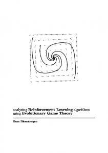
IV. E XPERIMENTS We performed experiments with five different maze tasks (one simple and four more complex problems) to compare the different ensemble methods to the individual algorithms. In the first experiment, the RL algorithms are combined with tabular representations and are compared on a small maze task. In the second experiment a partially observable maze is used and neural networks as function approximators. In the third experiment a dynamic maze is used where the obstacles are not placed at fixed positions and neural network function approximators are used. In the fourth experiment a dynamic maze is used where the goal is not placed at a fixed position and neural networks are used as function approximators. In the fifth and final experiment a generalized maze [23] task is used where the goal and the obstacles are not placed at fixed positions and again neural networks are used as function approximators. A. Small Maze Experiment The different ensemble methods: majority voting, rank voting, Boltzmann addition, and Boltzmann multiplication, are compared to the 5 individual algorithms: Q-learning, Sarsa, AC, QV-learning, and ACLA. We performed experiments with Sutton’s Dyna maze shown in Figure 1(A). This simple maze consists of 9 × 6 states and there are 4 actions; north, east, south, and west. The goal is to arrive at the goal state G as soon as possible starting from the starting state S under the influence of stochastic (noisy) actions. We kept the maze small, since we want to compare the results with the experiments on the more complex maze tasks, which would otherwise cost too much computational time. G
G
S
P
S
Fig. 1. (A) Sutton’s Dyna maze. The starting position is indicated by S and the goal position is indicated by G. In the partially observable maze of the second experiment the goal position is P and the starting position is arbitrary. (B) The 9 × 6 maze with dynamic obstacles used in the third experiment. The starting position is denoted by S and the goal position is indicated by G. The obstacles indicated in black are dynamically generated at the start of each new trial.
Experimental set-up. The reward for arriving at the goal is 100. When the agent bumps against a wall or border of the environment it stays still and receives a reward of -2. For other steps the agent receives a reward of -0.1. A trial is finished after the agent hits the goal or 1000 actions have been performed. The random replacement (noise) in action execution is 20%. This reward function and noise is used in all experiments of this paper. We used a tabular representation and first performed simulations to find the best learning rates, discount factors, and greediness (inverse of the temperature) used in Boltzmann exploration. All parameters were optimized for the single RL algorithms, where they were evaluated using the average reward intake and the final performance is optimized. Although
4
in general it can cause problems to learn to optimize the discounted reward intake while evaluating with the average reward intake, for the studied problems the dominating objective is to move each step closer to the goal, which is optimized using both criteria if the discount factor is large enough. We also optimize the discount factors, since we found that they had a large influence on the results. If we would have always used the same discount factor for all algorithms, the results of some algorithms would have been much worse, and therefore it would be impossible to select a fair discount factor. Since we evaluate all methods using the average reward criterion, the different discount factors do not influence the comparison between algorithms. The ensemble methods used the parameters of the individually optimized algorithms, so that only the ensemble’s temperature had to be set. TABLE I TABULAR LEARNING RATES α/β, DISCOUNT FACTOR AND GREEDINESS ( INVERSE OF THE TEMPERATURE FOR B OLTZMANN EXPLORATION ) FOR THE ALGORITHMS . T HE LAST FOUR COLUMNS SHOW FINAL AND CUMULATIVE RESULTS FOR THE TABULAR REPRESENTATION AND THE RANKS OF THE DIFFERENT ALGORITHMS ( SIGNIFICANCE OF T- TEST p = 0.05). R ESULTS ARE AVERAGES OF 500 SIMULATIONS . Method Q Sarsa AC QV ACLA+ Majority voting Rank voting Boltzmann mult Boltzmann add
α 0.2 0.2 0.1 0.2 0.005 – – – –
β – – 0.2 0.2 0.1 – – – –
γ 0.9 0.9 0.95 0.9 0.99 – – – –
G 1 1 1 1 9 1.6 0.6 0.2 1
5.14 5.26 5.21 5.25 5.20 5.33 5.01 5.34 5.28
± ± ± ± ± ± ± ± ±
Final 0.49 0.31 0.17 0.25 0.23 0.12 0.36 0.15 0.12
Rank 8 3-5 6-7 4-5 6-7 1-2 9 1-2 3-4
Cumulative 84.9 ± 11.5 90.3 ± 8.3 91.1 ± 3.3 91.4 ± 7.8 90.2 ± 5.2 96.7 ± 2.2 92.2 ± 7.9 95.3 ± 3.9 93.5 ± 1.9
Rank 9 5-8 5-7 4-7 7-8 1 4-5 2 3
In Table I we show average results and standard deviations of 500 simulations of the final reward intake during the last 2500 learning-steps and the total summed reward (adding all 20 average reward intakes after each 2,500 steps) during the entire trial lasting 50,000 learning-steps. This latter evaluation measure shows the overall performance and the learning rate with which good solutions are obtained. The ranks are computed using the student t-test with p = 0.05. Note that since 500 simulations were performed, small differences may still turn out to be significant. The results show that the majority voting and Boltzmann multiplication ensembles outperform all other methods. To show that the chosen discount factors matter, we also experimented with Sarsa with a discount factor of 0.95 and with ACLA using a discount factor of 0.9. Using the best found other learning parameters, Sarsa’s performance was 4.89 ± 1.14 for the final performance and 84.7 ± 20.0 for the total learning performance. Using the best other learning parameters, ACLA’s performance was 4.86 ± 0.86 for the final performance and 82.7±18.6 for the total learning performance. This clearly shows that care should be taken to optimize the discount factor if one wishes to compare different RL algorithms. All algorithms converge to a stable performance within 15,000 learning steps, but the best ensembles reach better performance levels and initially learn faster. B. Partially Observable Maze In this experiment we use Markov localization and neural networks to solve a partially observable Markov decision process in the case where the model of the environment is
known. We use Markov localization to track the belief state (or probability distribution over the states) of the agent given an action and observation after each time-step. This belief state is then the input for the neural network. We used 20 sigmoidal hidden neurons in our experiments, and the maze shown in Figure 1(A) with the goal indicated by P and each state can be a starting state. The initial belief state is a uniform distribution where only states that are not obstacles get assigned a non-zero belief. After each action at the belief state bt (s) is updated with the observation ot+1 : X bt+1 (s) = ηP (ot+1 |s) T (s′ , at , s)bt (s′ ) s′
where η is some normalization factor. The observations are whether there is a wall to the north, east, south, and west. Thus, there are 16 possible observations. We use 20% noise in the action execution and 10% noise for observing each independent wall (or empty cell) at the sides. That means that an observation is correct with probability 0.94 = 66%. Note that we use a model of the environment to be able to compute the belief state, and the model is based on the uncertainties in the transition and observation functions. TABLE II F INAL RESULTS ( AVERAGE REWARD FOR LAST 5,000 STEPS ) AND CUMULATIVE RESULTS FOR A NEURAL NETWORK REPRESENTATION ON THE PARTIALLY OBSERVABLE MAZE. R ESULTS ARE AVERAGES OF 100 SIMULATIONS . Method Q Sarsa AC QV ACLA+ Majority voting Rank voting Boltzmann mult Boltzmann add
α 0.02 0.02 0.02 0.02 0.035 – – – –
β – – 0.03 0.01 0.005 – – – –
γ 0.95 0.95 0.95 0.9 0.99 – – – –
G 1 1 1 1 10 1.4 0.8 0.2 1
9.65 9.41 9.33 9.59 8.44 9.37 9.30 9.56 9.11
± ± ± ± ± ± ± ± ±
Final 0.33 1.26 0.31 0.31 0.27 0.31 0.28 0.32 0.31
Rank 1-4 1-8 4-7 1-4 9 4-7 4-7 1-4 7-8
Cumulative 154.1 ± 7.3 137.6 ± 21.1 159.4 ± 3.5 135.3 ± 12.3 135.1 ± 3.7 139.8 ± 8.2 133.1 ± 13.3 174.6 ± 2.9 162.2 ± 2.6
Rank 4 5-9 3 6-9 6-9 5-6 6-9 1 2
We performed experiments consisting of 100,000 learning steps with a neural network representation and the Boltzmann exploration rule. For evaluation after each 5,000 steps we measured the average reward intake during that period. Table II shows that the Boltzmann multiplication ensemble method learns fastest in this problem. We also experimented with a Boltzmann multiplication ensemble consisting of five differently initialized Q-learning algorithms. The performance of this ensemble was 9.61 ± 0.31 for the final performance and 153.1 ± 8.0 for the total learning performance. This shows that combining different RL algorithms speeds up learning performance compared to an ensemble of the best single RL algorithm. All algorithms converge to a stable performance within 60,000 learning steps, but the best ensembles reach a good performance much earlier. C. Solving a Maze with Dynamic Obstacles We also compared the algorithms on a dynamic maze, where in each trial there are several obstacles at random locations (see Fig. 1(b)). In order to deal with this task the agent uses a neural network that receives as inputs whether a particular state-cell contains an obstacle (1) or not (0). The neural network uses 2 × 54 = 108 inputs including the position of the agent and 60 sigmoidal hidden units. At the start of each new trial there
5
are between 4 and 8 obstacles generated at random positions and it is made sure that a path to the goal exists from the fixed starting location S. Since there are many instances of this maze, the neural network has to learn the knowledge of a path planner. A simulation lasts for 3,000,000 learning steps and we measure performance after each 150,000 steps. TABLE III F INAL RESULTS ( AVERAGE REWARD FOR LAST 150,000 STEPS ) AND CUMULATIVE RESULTS FOR A NEURAL NETWORK REPRESENTATION ON THE MAZE WITH DYNAMIC OBSTACLES . R ESULTS ARE AVERAGES OF 50 SIMULATIONS . Method Q Sarsa AC QV ACLA+ Majority voting Rank voting Boltzmann mult Boltzmann add
α 0.01 0.01 0.015 0.01 0.06 – – – –
β – – 0.003 0.01 0.002 – – – –
γ 0.95 0.95 0.95 0.9 0.98 – – – –
G 1 1 1 0.4 6 2.6 0.8 0.2 1
6.79 6.66 5.98 6.27 5.39 6.93 6.59 7.04 6.08
± ± ± ± ± ± ± ± ±
Final 0.21 0.37 0.31 0.20 0.15 0.14 0.21 0.13 0.12
Rank 3 4-5 8 6 9 2 4-5 1 7
Cumulative 116.2 ± 2.7 112.6 ± 5.9 97.7 ± 9.4 108.3 ± 2.7 89.2 ± 1.3 122.1 ± 1.4 108.0 ± 2.6 125.0 ± 1.6 107.7 ± 1.3
Rank 3 4 8 5-7 9 2 5-7 1 5-7
Table III shows the final and total performance of the different algorithms. The Boltzmann multiplication ensemble outperforms the other algorithms on this problem: it reaches the best final performance and also has the best overall learning performance. We also experimented with a Boltzmann multiplication ensemble consisting of five differently initialized Q-learning algorithms. The performance of this ensemble was 6.87 ± 0.22 for the final performance and 117.0 ± 2.7 for the total learning performance. This shows again that combining different RL algorithms in an ensemble performs better than an ensemble consisting of the best single RL algorithm. The best ensembles reach a better performance at the end than the single RL algorithms. D. Solving a Maze with Dynamic Goal Positions In this fourth maze experiment, we use the same small maze as before (see Figure 1(A)) where the starting position is indicated by S, but now the goal is placed at a different location in each trial. To deal with this, we use a neural network function approximator that receives the position of the goal as input. Therefore there are 54 × 2 inputs, that indicate the position of the agent and the position of the goal. A simulation lasts for 3,000,000 learning steps and we measure performance after each 150,000 steps. We used feedforward neural networks with 20 sigmoidal hidden units. TABLE IV F INAL RESULTS ( AVERAGE REWARD FOR LAST 150,000 STEPS ) AND CUMULATIVE RESULTS FOR A NEURAL NETWORK REPRESENTATION ON THE MAZE WITH DYNAMIC GOAL POSITIONS. R ESULTS ARE AVERAGES OF 50 SIMULATIONS . Method Q Sarsa AC QV ACLA+ Majority voting Rank voting Boltzmann mult Boltzmann add
α 0.005 0.008 0.006 0.012 0.06 – – – –
β – – 0.008 0.004 0.006 – – – –
γ 0.95 0.95 0.95 0.95 0.98 – – – –
G 0.5 0.6 0.6 0.6 10 2.4 1.2 0.2 1
10.05 10.69 10.65 10.66 10.11 11.06 10.58 10.74 10.12
± ± ± ± ± ± ± ± ±
Final 0.37 0.47 0.11 1.16 1.80 0.06 2.08 0.06 0.09
Rank 7-9 2-7 3-7 2-7 3-9 1 2-7 2-5 7-9
Cumulative 152.7 ± 8.3 176.9 ± 8.7 180.5 ± 3.3 169.4 ± 20.2 121.5 ± 25.6 188.6 ± 2.1 82.4 ± 30.8 187.8 ± 1.9 170.7 ± 2.5
Rank 7 4 3 5-6 8 1 9 2 5-6
Table IV shows the final and total performance of the different algorithms. The majority voting ensemble outperforms the other algorithms on this problem: it reaches the
best final performance and also has the best overall learning performance. We also experimented with a majority voting ensemble consisting of five differently initialized Sarsa algorithms. The performance of this ensemble was 11.02 ± 0.22 for the final performance and 176.7 ± 4.9 for the total learning performance. This shows again that a combination of different RL algorithms in an ensemble learns faster than an ensemble consisting of the best single RL algorithm, although an ensemble of the same RL algorithm can also increase the final performance of that algorithm. The best ensembles reach a better performance at the end than the single RL algorithms and initially have a faster learning speed.
E. Solving the Generalized Maze In this last maze experiment, we use the same small maze as before, but now the goal and walls are placed at a different location in each trial. This is what Werbos calls the “Generalized Maze” [23] experiment. To deal with this, a neural network function approximator receives the position of the agent, goal and the dynamic walls as input. Therefore there are 54 × 3 inputs. A simulation lasts for 15,000,000 learning steps and we measure performance after each 750,000 steps. The feedforward neural networks have 100 sigmoidal hidden units. TABLE V F INAL RESULTS ( AVERAGE REWARD FOR LAST 750,000 STEPS ) AND CUMULATIVE RESULTS FOR A NEURAL NETWORK REPRESENTATION ON THE GENERALIZED MAZE . R ESULTS ARE AVERAGES OF 50 SIMULATIONS FOR THE SINGLE ALGORITHMS AND 10 SIMULATIONS FOR THE ENSEMBLES . Method Q Sarsa AC QV ACLA+ Majority voting Rank voting Boltzmann mult Boltzmann add
α 0.003 0.003 0.014 0.002 0.1 – – – –
β – – 0.0015 0.001 0.001 – – – –
γ 0.95 0.92 0.95 0.95 0.98 – – – –
G 0.3 0.3 0.5 0.2 5 2.4 1.0 0.2 1
6.92 1.06 5.84 5.17 4.81 6.68 6.02 6.54 5.65
± ± ± ± ± ± ± ± ±
Final 0.16 0.20 0.15 0.16 0.12 0.23 0.16 0.13 0.14
Rank 1 9 5 7 8 2-3 4 2-3 6
Cumulative 96.6 ± 1.1 13.3 ± 0.9 89.0 ± 1.0 76.6 ± 1.1 56.7 ± 1.5 102.6 ± 0.8 48.6 ± 2.2 100.8 ± 1.0 86.0 ± 0.8
Rank 3 9 4 6 7 1 8 2 5
Table V shows the final and total performance of the different algorithms. Here Q-learning obtains the best final results, but the majority voting ensemble has the best overall learning performance. It is surprising that Sarsa obtains much worse results than the other algorithms, even though we optimized all its learning parameters. We also experimented with a majority voting ensemble consisting of five Q-learning algorithms. The performance of this ensemble was 7.20 ± 0.16 for the final performance and 103.4±0.9 for the total learning performance, so this ensemble reaches the best final performance, and its learning speed is almost significantly better than the majority voting ensemble using different RL algorithms. This is the only experiment where an ensemble consisting of the same best single RL algorithm leads to a significantly better final performance compared to the best ensemble consisting of different single RL algorithms. This results can be explained by the fact that in this problem Q-learning performs much better than the other algorithms. At the end of the learning trial Q-learning outperforms the best ensembles, although the ensembles initially have a faster learning speed.
6
V. D ISCUSSION From the results it is clear that the Boltzmann multiplication (BM) and majority voting (MV) ensembles significantly outperform the other methods in terms of final performance. The Boltzmann multiplication (BM) ensemble significantly outperforms the other methods in terms of total learning performance and the majority voting method comes as second best. The rank voting and Boltzmann addition ensembles do not outperform single RL algorithms. The results showed that the best ensemble always learns fastest, but one may have noticed that the ensembles cost more computational time. Although this is true, many real world scenarios such as robotics require the least number of experiences, since the actions taken in real time require much more time than the actual calculation done by the learning algorithms. Furthermore, in all experiments, the best ensemble has a better or equal final performance compared to the best single RL algorithm. Even in the generalized maze, the ensemble consisting of five Q-learning algorithms outperforms the single Q-learning algorithm. Experiments also showed that an ensemble with different RL algorithms often outperforms an ensemble consisting of the best RL algorithm, even though some RL algorithms perform considerably worse. This is due to the fact that ensembles improve independent algorithms most if the algorithms’ predictions are less correlated. We think that good ensemble algorithms outperform single RL algorithms because the ensemble can make a better trade-off between exploration and exploitation by determining action choices based on the uncertainties of all algorithms. If the algorithms want to choose the same action, it is more likely that this action will be exploited than when algorithms disagree. In future work we want to focus on batch [10] and modelbased RL algorithms [9], which can be very useful for reducing the number or experiences. We are also currently studying methods for learning to weigh each independent RL algorithm, which could increase the performance of the ensembles even further. Finally, we want to compare all algorithms on the partially observable generalized maze problem.
[8] J. Baxter and P. Bartlett, “Infinite-horizon policy-gradient estimation,” Journal of Artificial Intelligence Research, vol. 15, pp. 319–350, 2001. [9] A. W. Moore and C. G. Atkeson, “Prioritized sweeping: Reinforcement learning with less data and less time,” Machine Learning, vol. 13, pp. 103–130, 1993. [10] M. Riedmiller, “Neural fitted Q iteration - first experiences with a data efficient neural reinforcement learning method,” in Proceedings of the Sixteenth European Conference on Machine Learning (ECML’05), 2005, pp. 317–328. [11] L. Breiman, “Bagging predictors,” Machine Learning, vol. 24, no. 2, pp. 123–140, 1996. [12] Y. Freund and R. E. Schapire, “Experiments with a new boosting algorithm,” in Proceedings of the thirteenth International Conference on Machine Learning. Morgan Kaufmann, 1996, pp. 148–156. [13] R. A. Jacobs, M. I. Jordan, S. J. Nowlan, and G. E. Hinton, “Adaptive mixtures of local experts,” Neural Computation, vol. 3, no. 1, pp. 79–87, 1991. [14] S. P. Singh, “The efficient learning of multiple task sequences,” in Advances in Neural Information Processing Systems 4, J. Moody, S. Hanson, and R. Lippman, Eds. San Mateo, CA: Morgan Kaufmann, 1992, pp. 251–258. [15] C. Tham, “Reinforcement learning of multiple tasks using a hierarchical CMAC architecture,” Robotics and Autonomous Systems, vol. 15, no. 4, pp. 247–274, 1995. [16] R. Sun and T. Peterson, “Multi-agent reinforcement learning: weighting and partitioning,” Neural Networks, vol. 12, no. 4-5, pp. 727–753, 1999. [17] D. Ernst, P. Geurts, and L. Wehenkel, “Tree-based batch mode reinforcement learning,” Journal of Machine Learning Research, vol. 6, pp. 503–556, 2005. [18] C. J. C. H. Watkins and P. Dayan, “Q-learning,” Machine Learning, vol. 8, pp. 279–292, 1992. [19] R. S. Sutton, “Learning to predict by the methods of temporal differences,” Machine Learning, vol. 3, pp. 9–44, 1988. [20] K. S. Narendra and M. A. L. Thathatchar, “Learning automata - a survey,” IEEE Transactions on Systems, Man, and Cybernetics, vol. 4, pp. 323–334, 1974. [21] J. A. Boyan and A. W. Moore, “Generalization in reinforcement learning: Safely approximating the value function,” in Advances in Neural Information Processing Systems 7, G. Tesauro, D. S. Touretzky, and T. K. Leen, Eds. MIT Press, Cambridge MA, 1995, pp. 369–376. [22] G. Gordon, “Stable function approximation in dynamic programming,” Carnegie Mellon University, Tech. Rep. CMU-CS-95-103, 1995. [23] P. Werbos and X. Pang, “Generalized maze navigation: Srn critics solve what feedforward nets cannot,” IEEE Transactions on Systems, Man, and Cybernetics, vol. 3, pp. 1764–1769, 1996.
R EFERENCES [1] R. S. Sutton and A. G. Barto, Reinforcement Learning: An Introduction. The MIT press, Cambridge MA, A Bradford Book, 1998. [2] L. P. Kaelbling, M. L. Littman, and A. W. Moore, “Reinforcement learning: A survey,” Journal of Artificial Intelligence Research, vol. 4, pp. 237–285, 1996. [3] C. J. C. H. Watkins, “Learning from delayed rewards,” Ph.D. dissertation, King’s College, Cambridge, England, 1989. [4] G. Rummery and M. Niranjan, “On-line Q-learning using connectionist sytems,” Cambridge University, UK, Tech. Rep. CUED/F-INFENG-TR 166, 1994. [5] R. S. Sutton, “Generalization in reinforcement learning: Successful examples using sparse coarse coding,” in Advances in Neural Information Processing Systems 8, D. S. Touretzky, M. C. Mozer, and M. E. Hasselmo, Eds. MIT Press, Cambridge MA, 1996, pp. 1038–1045. [6] M. Wiering and H. van Hasselt, “Two novel on-policy reinforcement learning algorithms based on TD(λ)-methods,” in Proceedings of the IEEE International Symposium on Adaptive Dynamic Programming and Reinforcement Learning, 2007, pp. 280–287. [7] R. Sutton, D. McAllester, S. Singh, and Y. Mansour, “Policy gradient methods for reinforcement learning with function approximation,” in Advances in Neural Information Processing Systems 12. MIT Press, 2000, pp. 1057–1063.
PLACE PHOTO HERE
PLACE PHOTO HERE
Marco Wiering Dr. Marco Wiering finished his Ph.D. with the topic reinforcement learning in 1999. From January 2000 until September 2007 he was an assistant professor at University Utrecht. He is now pursuing a tenure track at the university of Groningen in the field of cognitive robotics. Dr. Wiering is mostly researching the fields of machine learning, especially reinforcement learning, robotics, and machine vision.
Hado van Hasselt Hado van Hasselt obtained a Master degree in Cognitive Artificial Intelligence at the University of Utrecht in 2006, where he is currently a Ph.D. student at the Intelligent Systems Group of the Department of Information and Computing Sciences. Hado van Hasselt is interested in machine learning, reinforcement learning, and handwritten text recognition.