Evaluation of a Hierarchical Partitioned Particle Filter with Action Primitives Zsolt L. Husz Joint Research Institute in Signal and Image Processing, EPS Heriot-Watt University, Edinburgh
Andrew M. Wallace Joint Research Institute in Signal and Image Processing, EPS Heriot-Watt University, Edinburgh
[email protected]
[email protected]
Patrick R. Green School of Life Sciences Heriot-Watt University, Edinburgh
[email protected]
Abstract
to use multiple views. For an overview of human action recognition and tracking [1] and [11] can be consulted. Deutscher et al. [3] used an annealed particle filter (APF) with dynamic hierarchical partitioning. This is similar to our approach, but we use fixed partitions determined by the human body structure. Multiple modes in the parameter space make it inappropriate to use unimodal co-variances to define the partitions. MacCormick et al. [10] partitioned the parameter space, tracking parameters independently. They argued that partitioned sampling is the equivalent of hierarchical search. Their partitioning is valid only if the parameters are independent or loosely independent. However, we argue that when high, hierarchic dependence is present, as for the human body, then simple partitioning is not practical. The Hierarchical Partitioned Particle Filter (HPPF) performs a stochastic search in a high dimensional space, converging through several predefined levels to the solution. The difficulty of 3D human tracking arises from the complexity of the human body that is a search of a high dimensional space with limited data. HPPF offers a natural solution, first embedding the structure of the tracked object and second providing prior and likelihood integration on multiple levels. Although HPPF can be viewed as a mixture of the APF [3] and partitioned particle filter [10] there are important differences. The earlier work takes no account of the hierarchical dependency between parameters which is essential to properly model dynamics of the articulated human body. Further, we integrate priors on multiple levels sequentially, performing guided annealing to escape from local minima. The search in the high dimensional space is inefficient without an additional prior model directing the search. We use a switching model, which combines the usual Gaussian
We introduce the Hierarchical Partitioned Particle Filter (HPPF) designed specifically for articulated human tracking. The HPPF is motivated by the hierarchical dependency between the human body parameters and the partial independence between certain of those parameters. The tracking is model based and follows the analysis by synthesis principle. The limited information of the video sequence is balanced by prior knowledge of the structure of the human body and a motion model. This is based on action primitives, a sequence of consecutive poses, each predicting in a stochastic manner the next pose. Tracker performance is evaluated on the HumanEva-II dataset for different motion model parameters, number of camera views and particles.
1. Introduction Motion capture, the analysis of human activity, and the understanding of behaviour have attracted an increasing interest in surveillance, entertainment, intelligent domiciles and medical diagnosis. Human tracking [5, 7] is the initial phase of most behavioural analysis. It is possible to track human bodies as a whole [6], considering them as blobs, or as articulated objects [3, 4, 9, 14], fitting a humanoid structure. The former approach has the advantage of simplicity, fast algorithms, applicability to single or multiple views, and robustness, but the information extracted is limited and only simple classification can be performed[6]. Tracking articulated objects [3, 14, 12] needs complex, high dimensional models and algorithms that are generally slow. Further, as the result is more complex, it may be necessary 1
Particle update
Weight and resample
6D
Level 1
Torso
Initial particle set
Motion updated particles
Selected and re− sampled particles
Recobination 1 2D
Repeat on the next level i−th level
Left upper arm
2D
Right upper arm
2D
Left upper leg
2D
Right upper leg
2D
Head
6D
Torso
Level 2
Recobination 2
Repeat on the next frame
Global evaluation 2D
Globally fitted particles
Figure 1. HPPF structure: evolution of the particle set on multiple levels, followed by global evaluation and resampling. On each level particles are updated by a probabilistic prior motion model and evaluated by the likelihood function.
noise model with action primitives predicting the next pose on the basis of the previous poses. This model uses the learnt motion to reduce the search space, but still allows the possibility of previously unseen movement.
2. Hierarchical Partitioned Particle Filter In the particle filter (PF) approach, the density estimate of the current state is represented either by the mean or by the mode of a set of particles, each a full set of parameters of the state. For a new observation the particles are updated using the priors and the measurement based likelihoods. When the parameters are inter-dependent, it is natural to adapt the PF to a hierarchy in which for each new observation a particle goes through levels of filtering; each level adjusts sets of inter-dependent parameters and the other parameters are only slightly affected if at all. A limited number of iterations is applied, equal to the number of the levels. Partitioning exists both between levels, adjusting different groups of parameters; and on each level, adjusting in parallel independent parameters. This is the basic idea behind the HPPF. The HPPF has an iterative phase for each level (Figure 1), consisting of three sequential steps: motion update, weight evaluation and particle re-sampling. On the first level the most independent parameters (i.e. global positions) are adjusted, then the hierarchical inferior parameters (the upper then the lower limbs). Parameters on level 2 and 3 (of the four limbs) are physically independent therefore these parameter partitions are independently evaluated and propagated. (The independence of the limbs is arguable; for some activities (walk, jog) the limbs are highly correlated, but for unrestricted activity they are independent.) Final global evaluation and re-sampling keeps the best global solutions generated from the mixing of good local solutions and computes the mean of the particles that are similar with the mode of the particles only. This mean proposes to reduce the effect of a mean on a multi-modal distribution. The three levels of the HPPF applied to the human body model are shown in Figure 2.
Left lower arm
2D
Right lower arm
2D
Left lower leg
2D
Right lower leg
Torso,
16D
Upperlimbs,
Level 3
Head Recobination 3 Global evaluation
Figure 2. HPPF applied to human tracking for one frame first modifies the global, torso parameters; followed by the upper limb and head, and finally by the lower limb parameters. Each body part forms a partition, while the last partition on level 2 and 3 contain higher level parameters slightly tuned to fit the lower level body parts. The global evaluation evaluates the whole particle.
The particle update updates the particles based on the motion model explained in Section 3. The weight evaluation and global evaluation assess each particle independently with the weighting function (the unnormalised posterior), given by Bayes rule w(px |I) = Ω(px ) · Λ(I|px ).
(1)
px is a parameter sub-set of particle p defined by the evaluated partition x of the current level or, for global evaluation, x is the full parameter set of p. In the later case the p notation will be used for px . Ω(px ) is the prior for px , based on physical range of the parameters, being 1 in the the nominal range and exponentially decaying outside this range. Λ(I|px ) is the likelihood for image I, both partition level and global likelihoods are discussed in section 4. The global evaluation selects with the MAP estimate the best fitting particles from the globally weighted particles. For particle re-sampling, PFs usually use systematic resampling [2, p. 42] to solve the particle set degeneracy problem. In addition to degeneracy in a high dimensional space the number of required particles for a good density estimate increases exponentially [3, 10]. While particle set degeneration [2] is not desired, only viable particles must propagate to the next level, but preserving the multi-modality and variety. In our modified basic systematic re-sampling, only the highest 80% of particles survive. This is required by parameters which are badly characterised by the likelihood function (e.g. due to depth ambiguity, occlusions, low contrast) alowing surival of poorly matching particles with relatively high weights. Particles are re-sampled per partition basis, sets of parameters are weighted by the likelihood of their partition. This inherently can mix lower and higher level parameters, and combination might result in a global configura-
tion with low likelihood. This is partly solved by slight variations of the higher level parameters at a lower level, assuring their stability and as result the mixing degradation is avoided. This mixing is essentially the same as the crossover operation between particles beneficial to the APF approach [3]. The global evaluation integrates the level based adjustments, therefore solves mixing problems.
by expectation maximisation. For each cluster the mean and covariance of the member APs of the first D BFV are computed as well as the mean and covariance of the last BFV, which is the NBFV for the length D AP. The stages of the APCs learning algorithm are described in [8]. The similarity of an unknown ap action primitive with an APC χ is ′
The underlying articulated human model consists of 10 body parts, each modelled by a truncated frustum with constant elliptical subsection and heights. The body parts have constant lengths and the body configuration is completely defined by 24 parameters, including the body root position, the body orientation, spline tilt and azimuth, and the 18 joint angles. This model allows a compact representation of a pose by the 24 parameter vector. However it differs from the HumanEva model: each joint rotation, defined by its nature, is parametrised by 1, 2 or 3 Euler angles, while in HumanEva it is parametrised by a 4 × 4 transformation matrix. The gimbal lock restrains the recovery of the Euler angles and HumanEva data shows two DOF compared to the single DOF we assume. Our model has constant body size, while HumanEva allows varying size. HumanEva MOCAP data also has impossible leg poses, with knees bent backward (e.g. pose of right leg in S1 Walking 1 sequence, around frame no.620). Due to the model differences the mean 3D/2D error of the converted HumanEva training data to our model is 23mm/3pixel. A body feature vector (BFV) is a set of the parameters describing a body configuration, having as elements either direct features (joint angle, body position, orientation) or features derived by simple operations from direct features (velocity, global position vector). We use a set of 14 different BFVs each with direct features: the 18 joint angles describing the whole body configuration; four subsets each with four joint angles of each limb; one for the head with two joint angles; and eight subsets with two joint angles for each of the lower and higher limbs. The 14 BFVs result in 14 motion models used to update parameters partitioned at different levels of the HPPF. An action denotes a short, variable length sequence of body configuration (e.g. leg rising, arm still) and is defined by one or more body parts. The action primitive model (APM) uses action primitives (AP), basic actions, parts of the larger time-scale actions, represented by a sequence of consecutive BFVs. The APM predicts the next body feature vector (NBFV) for each AP. An AP is a set of consecutive BFV, therefore it captures both the static and the dynamic behaviour of the BFVs. The APM consists of action primitive clusters (APC), a group of similar APs. For this, the principal component analysis compressed APs of original length D+1 BFV, are clustered
−1
simχ (ap) = eδ(ap) ∗Σχ
3. Motion Model
∗δ(ap)
(2)
where Mχ and Σχ are the precomputed mean and covariance of the PCA compressed cluster χ and δχ (ap) = Mχ − ap ˆ
(3)
is the difference from the cluster mean and the PCA projected ap. ˆ The highest similarity results in the best matching cluster γ(ap) = argmaxχ∈X simχ (ap)
(4)
If px is a subset of particle parameters the prediction of its next state is given by the ap = F (px )
(5)
which constructs the AP from the set of the parameters of px and tracking results in the previous frames. Using the best of the parameter set matching γ(F (p)) the next values pk+1 x are determined stochastically by pk+1 = MN BF V (γ(ap)) + H ∗ ΣN BF V ∗ E x
(6)
or ∗ ∗ pk+1 = pkx + MN x BF V (γ(ap)) + H ∗ ΣN BF V ∗ E
(7)
with H a heating constant, and E a standard Gaussian white noise error vector. MN BF V and ΣN BF V are the mean and ∗ ∗ covariances of all NBFVs, and MN BF V and ΣN BF V the mean and covariance of the difference between NBFV and previous BFV in the APC γ(ap). To train the above parameters of each APC the full HumanEva-I dataset train MOCAP sequences were used. The frequently used motion model [3] pk+1 = pk + B
(8)
adds Gaussian noise B to the current particle parameters. The tracked model is human, therefore the motion is highly constrained. To maintain the model generality, but restraining the model, our motion can switch between random added noise of (8) and the AP based models defined in (7) and (6) with equal probabilities. The main feature of the APM is the reduction of the motion to a structure similar to a Hidden Markov Model (HMM). However, a HMM state is
a discrete random variable, while, for the APM, a particle is a vector of continuous random variables. While transitions in HMM directly define the next discrete state and its probability, for the APM a transition generates individual continuous values of each of the parameters. This is done first, by mapping the current AP into an APC, reducing the set of continuous parameters to a single random variable, the cluster number; then generating explicitly the new AP in the continuous domain by replacing the oldest BFV in the AP with a newly generated NBFV from the precomputed mean and the covariance of the current APC. (Figure 3).
S3 S4
S1
S2
S6 S5 S7
Figure 3. Visual representation of the APM. A discrete APC is shown as a smaller continuous circle Si. This APC transforms transforms into a new BFV generated by the mean and covariance, shown as larger dotted circle, of the NBFV. The NBFV and the current AP results in the new AP, which is assigned to a discrete APC. S1 transforms into S3 or S4; S2 transforms into S1 or stays in the same state (but changes the parameter values); S3 to S3 or S4; S4 to S5, S6 or S7; S5 to S4;S6 to S1 or S2; and S7 to S5 , S6 or S7. Any transition will result in some changes of the continuous parameters.
4. Likelihoods The λx (I|px ) likelihood of the image I given the parameter partition px of one or more body parts x is based on the match of the projected 3D parts to the input image. For simplicity we omit I and represent λx (I|px ) = λx (px ). Perspective projection of equally sampled points of the body part frustums onto the image are the measurement points. Self occlusion of different body parts is solved by a method similar to the Z-buffering, by ordering the depth of the centres.
4.1. Partition likelihood The partition based likelihood λx (px ) is computed for each partition of each level as the product of the body part based likelihoods. λx (pi ) of each body part is defined by
the partition parameters, i, a subset x. λx (pi ) of each body part are considered independent observations, therefore their product gives λx (px ). The λx (pi ) is provided by the edge, the silhouette (foreground) and the colour likelihoods. Self occlusion is solved by the combination of the likelihood, called the matching Mi , of the image (edge, silhouette or colour) and the projected estimate; and the body part relevance, Ri . The relevance acts as a prior on the likelihood measured by Mi and is computed based on the visibility of the body part. The likelihood of a body part i on level l is λx (pi ) = eRi ∗log(Mi ) . (9) We use silhouette and edge based matches, each defined by the percentage of the sampled internal or edge points of the projected body having a match in the foreground or in the Sobel edge map. In comparison with the Deutscher and Reid [3] likelihood, that is a global likelihood for the whole body, the used likelihood is body part. The colour based matches are obtained by the Bhattacharyya distance from the original body part colour histogram. The relevances are computed as the percentage of sampled measurement points not occluded by other parts. Silhouette, edge and colour relevances and matchings are combined with equal weights, resulting in the body part match and relevance Mi and Ri and with (9) the likelihood λx (pi ).
4.2. Global likelihood The alignment likelihood at the global evaluation level, countmismatch alg countnon background
−σ1
λG (p) = e
(10)
is computed in the bounding box of the projected model defined by particle p. The likelihood measures how the projected model overlaps the foreground silhouette, computed in the bounding box of the projected model extended in each direction by 25% in length. The countmissmatch is the number of image foreground pixels which have no overlapped projected model, ideally and countnon background the number of pixels which are either silhouette or projected model pixel; and σalg = 0.25. While partition likelihoods tend to cover all projected pixels with silhouettes, λG (p) is maximised when all silhouette pixels are matched with the projected model, having adverse effects.
5. Tracking results The effect of number of the clusters and sequence length of the APM; the number of particles and the number of camera views are analysed. For this the HumanEva-II Subject S2, Combo Action, Trial 1 dataset, with 4 camera views and Subject S1, Walk, Validate dataset with 1 to 3 views are used. The mean errors for the three frame-sets were computed by the means of the on-line evaluation system [13].
D 3
15
25
C 20 60 80 100 20 60 80 100 20 60 80 100
Set 1 121.9 99.99 114.1 94.91 105.1 110.7 114.2 128.5 101.9 130.8 108.8 117.0
Set 2 113.7 103.3 114 100.6 106 110.1 111.5 129.7 104.9 128.3 110.0 115.7
Set 3 137.7 140.0 149.4 136.4 147.1 136.1 148.6 172.3 155.4 155.0 151.2 143.0
Table 1. 3D relative tracking error [mm] for S2 Combo 1 sequence for number of clusters C = 20, 60, 80, 100 and length of sequence D = 3, 15, 25
Both the tracking and training data is sub-sampled to 20fps, therefore the tracking processes every third image and APM is trained with 6 individual sequences subsampled from each of the original 120fps MOCAP data sequences of the HumanEva-I dataset. The tracking algorithm requires initialisation provided by the HumanEva-II dataset. The un-optimised code requires approximately 85ms/(f rame ∗ particle) using four views on a P4 2.4GHz workstation with 1GB RAM with I/O through network. The tracking code does not include visualisation and uses preprocessed Sobel edge images, with 0.02 threshold, and foreground images resulted from background subtraction [15].
5.1. Motion model parameters Table 1 compares the effect of the motion model cluster number C and sequence length D effect on the tracking. Having low D results in short motion memory, while high D results in long motion memory. The low C restricts the number of APs, and therefore the estimation of the current AP is less accurate and the prediction of the next pose is inferior. Longer sequence length requires more APCs to fit each longer AP well. Better results for a short AP are unexpected, however they are explained by the fact that the next pose can be defined by the previous few poses; the good estimates in the previous poses over D frames are another requirement, harder to maintain for a larger D and if the APCs are overspecialised. Table 1 shows the best tracker performance with C = 100 and sequence length D = 3.
5.2. Number of particles Increasing the number of the particles leads to a better density estimate of the possible poses. This is expected and Table 2 confirms that higher particle numbers reduce the 3D tracking error, however above 200-500 particles the en-
P 50 100 200 500 1000
Set 1 139.0 156.7 114.1 108.6 102.7
Set 2 129.4 137.9 114.0 104.6 102.6
Set 3 154.1 155.6 149.4 128.8 133.0
Table 2. 3D relative error[mm] for S2 Combo 1 sequence for number of particles P = 50, 100, 200, 500, 1000, with C = 80 and D=3
hancements are not significant and do not justify the higher processing times.
5.3. Number of camera views An aim of a human motion model is to impose a priori knowledge in addition to the image-based observations. Ideally, with a good motion prediction a single or few views will provide good observations. Here, we analyse the effect of reducing the number of the cameras on the S1 Walking 1 sequence frames 6–590. Table 3 shows that for multiple cameras (two or three) the relative and absolute errors are similar, therefore the pose is well estimated. With two cameras, the 3D tracking error is 42% greater than with three. With a single camera, the lower relative than absolute 3D error suggests that the poses are better recovered, while the 3D positions are poorly recovered, because the depth is recovered only from the scale variations of the projected model.
5.4. Other sequences Providing comparison data with other methods, we run the tracking (P = 200 particles, C = 80 clusters of length D = 3) with the three test HumanEva-II sequences. Results with the 3D and 2D relative errors are shown in Table 4. Figures 4 and 5 show initial and intermediate frames of tracking for the S1 Walk and S2 Combo sequences1 . The general position and orientation of the human body is well tracked during all sequences. For the Walk sequence, the legs are tracked well, but after frame no. 160 the lower arms are lost and recovered just partially. Problems tracking the lower arms are in both the Combo sequences, but they recover with better observations. In the Combo sequences both walking and jogging leg motions are well recovered, and even during jogging, the slight centrifugal inclination toward the centre of the walking area is recovered, and is visible in the 3D reconstructions. The balancing activities are also recovered with slight errors. The errors of the unseen S4 Combo sequence are comparable to the sequences of the trained subjects, suggesting a similar performance for other unseen activities. 1 Videos of the full 3D reconstruction and projected camera C1 and C2 views are available at http://www.ece.eps.hw.ac.uk/˜zlh1/EHuM2/videos
Frame 9
Frame 12
Frame 15
Frame 18
Frame 21
Frame 24
Frame 27
Frame 30
Frame 33
Frame 36
Frame 219
Frame 225
Frame 231
Frame 237
Frame 243
Frame 246
Frame 249
Frame 252
Frame 255
Frame 258
Figure 4. The recovered pose back projected to the view of camera C1 (above) and the corresponding 3D pose (below) for the S1 Walk 1 sequence, frames 9–36 and 219–258 (3 frame step size).
Frame 4
Frame 7
Frame 10
Frame 13
Frame 16
Frame 19
Frame 22
Frame 25
Frame 28
Frame 31
Frame 451
Frame 454
Frame 457
Frame 460
Frame 463
Frame 466
Frame 469
Frame 472
Frame 475
Frame 478
Figure 5. The recovered pose back projected to the view of camera C1 (above) and the corresponding 3D pose (below) for the S2 Combo 1 sequence, frames 4–31 and 451–478 (3 frames step size).
Cameras C1,C2,C3 C1,C2 C1 C2
3D error[mm] 105.7/105.7 140.9/130.2 224.5/811.7 234.2/665.7
C1 error[pixel] 14.8/14.8 18.3/17.3 34.3 /38.6 34.7/119.4
C2 error[pixel] 14.8/14.7 19.4 / 18.6 32.2/145.6 31.0/29.8
Table 3. 3D relative/absolute tracking errors for S1 Walk 1 sequence frames 6-590, for P = 200 particles, C = 80 and D = 3. The 3D error and the 2D errors projected onto camera 1 and camera 2 views for all three, and both or one of the camera 1 and the camera 2 views.
Sequence S2 Combo 1 S4 Combo 4 S1 Walking 1
Set 1 114.1 179.8 101.9
3D[mm] Set 2 Set 3 114 149.4 153.1 156.6 N/A N/A
3D/2D error Camera 1[pixel] Set 1 Set 2 Set 3 15.2 14.5 21.43 28.94 22.99 23.39 14.01 N/A N/A
Camera 2[pixel] Set 1 Set 2 Set 3 15.8 15.5 18.13 25.62 20.41 20.42 14.18 N/A N/A
Table 4. 3D and 2D relative tracking error[mm] for the three HumanEva 2 test sequences.
6. Discussion and conclusions The Hierarchical Partitioned Particle Filter tracks articulated, high dimensional structures with hierarchical dependence between the parameters. The HPPF uses a motion based on Action Primitives, predicting next possible poses based on a history of previous poses. We have presented the HPPF results on the three EHuM2 evaluation datasets. Although not evaluated, we expect the tracker will perform equally well on any other HumanEva sequence as it is trained with all of the motions present in HumanEva dataset. We have to emphasise that motion is not constrained to the activities present in the evaluation set. Unexpected, a longer motion memory of the action primitives does not improve the tracking. Higher particle numbers, up to around 500 particles, improves the results, but further increase does not result in additional improvement. Lower arm errors could be fixed with enhanced likelihood functions and code optimisation would greatly increase the processing speed and would permit a higher number of particles resulting in better accuracy. In the larger context[8], the tracking with APs is important as it provides behavioural information about the action performed by the tracking subject. Full integration of tracking and behaviour analysis will be evaluated in the near future.
References [1] J. K. Aggarwal and S. Park. Human motion: Modeling and recognition of actions and interactions. In Proc. 2nd Int’l Symp. on 3D Data Processing, Visualization and Transmission, pages 640–647, 2004. 1 [2] N. G. Branko Ristic, Sanjeev Arulampalam. Beyond the Kalman Filter: Particle filters for tracking applications. Artech House Publishers, 2004. 2 [3] J. Deutscher and I. D. Reid. Articulated body motion capture by stochastic search. International Journal of Computer Vision, 61(2):185–205, Feb. 2005. 1, 2, 3, 4 [4] P. F. Felzenszwalb and D. P. Huttenlocher. Pictorial structures for object recognition. International Journal of Computer Vision, 61(1):55–79, 2005. 1
[5] D. Gavrila. The visual analysis of human movement: A survey. Computer Vision and Image Understanding, 73(1):82– 98, Jan. 1999. 1 [6] I. Haritaoglu, D. Harwood, and L. S. Davis. W4: Realtime surveillance of people and their activities. IEEE Trans. Pattern Analysis and Machine Intelligence, 22(8):809–830, 2002. 1 [7] W. Hu, T. N. Tan, L. Wang, and S. J. Maybank. A survey on visual surveillance of object motion and behaviors. IEEE Transactions on Systems, Man and Cybernetics, 34(3):334– 352, Aug. 2004. 1 [8] Z. L. Husz, A. M. Wallace, and P. R. Green. Human activity recognition with action primitives. In Proc. IEEE Int’l Conf. on Advanced Video and Signal-based Surveillance, Sept. 2007. 3, 8 [9] M. W. Lee and I. Cohen. Human body tracking with auxiliary measurements. In Proceedings of the IEEE International Workshop on Analysis and Modeling of Faces and Gestures (AMFG), pages 112–119, 2003. 1 [10] J. MacCormick and M. Isard. Partitioned sampling, articulated objects, and interface-quality hand tracking. In Proc. European Conf. on Computer Vision, LNCS, pages II: 3–19, 2000. 1, 2 [11] T. B. Moeslund, A. Hilton, and V. Kruger. A survey of advances in vision-based human motion capture and analysis. Computer Vision and Image Understanding, 103(2-3):90– 126, Nov. 2006. 1 [12] L. Sigal, S. Bhatia, S. Roth, M. J. Black, and M. Isard. Tracking loose-limbed people. In Proc. IEEE Conf. on Computer Vision and Pattern Recognition, pages 421–428, 2004. 1 [13] L. Sigal and M. J. Black. HumanEva: Synchronized video and motion capture dataset for evaluation of articulated human motion. Technical Report CS-06-08, Brown Univ., 2006. 5 [14] C. Sminchisescu and B. Triggs. Covariance scaled sampling for monocular 3D body tracking. In Proc. IEEE Conf. on Computer Vision and Pattern Recognition, volume 1, pages 447–454, 2001. 1 [15] C. Stauffer and W. E. L. Grimson. Adaptive background mixture models for real-time tracking. In Proc. IEEE Conf. on Computer Vision and Pattern Recognition, pages 246–252, 1999. 5