Sep 6, 2000 - continuously varying flow fields by means of digital ... Lawson et al. (1999) used a ... dynamic flow processes under a compression stroke of a.
Experiments in Fluids 30 (2001) 537±550 Ó Springer-Verlag 2001
Evaluation of transient turbulent flow fields using digital cinematographic particle image velocimetry S. Y. Son, K. D. Kihm
Abstract This paper describes an experimental development for temporal and spatial reconstruction of continuously varying ¯ow ®elds by means of digital cinematographic particle image velocimetry (PIV). The system uses a copper-vapor laser illumination synchronized with a high-speed camera, and continuously samples at 250 fps to measure transient and non-periodic turbulent ¯ows with relatively low frequencies, i.e., the surf zone turbulence produced by depth-limited wave break in a long laboratory ¯ume. The use of the developed PIV system comprehensively records the temporal development of both phase-averaged and instantaneous turbulent vortex ¯ows descended from the breaking waves to the bottom. Also, the measured power spectra show harmonic frequencies, ranging from the orbital frequency of 0.5 Hz up to the order of 5 Hz, and the well-known )5/3 dependence upon the turbulence ¯uctuation frequencies thereafter.
1 Introduction The particle image velocimetry (PIV) technique has become a fast-growing attraction in measuring ¯ow velocity ®elds, primarily due to its breakthrough advantage of whole-®eld mapping capability over the traditional singlepoint measurement probes. Extensive bibliography of the literature on PIV development is available from several review publications (e.g., Adrian 1996; Raffel et al. 1998). The recent development of a cross-correlation CCD camera, synchronized with pulsed Nd:YAG laser illumination, allows suf®ciently fast recording of two consecutively time-tagged images, which alleviates the ¯ow direction ambiguities occurring in the case of autocorrelation of superimposed images on a single frame (Adrian 1986). This also eliminates the image-biasing problem caused by the image shift when using a rotating Received: 2 December 1999/Accepted: 6 September 2000
S. Y. Son, K. D. Kihm (&) Department of Mechanical Engineering Texas A and M University College Station, TX 77843-3123, USA The authors gratefully acknowledge the NSF-sponsored Offshore Technology Research Center (OTRC) of Texas A and M University, for providing funding for the development and use of the digital cinematographic PIV system. The authors would like to thank Dr. D. Cox of Civil Engineering at Texas A and M University for his technical help in running the two-dimensional ¯ume to generate two-dimensional breaking waves.
mirror arrangement (Raffel and Kompenhans 1995; Lee et al. 1996). In addition, the unprecedented advancement of computer technology makes it possible to handle and process excessive amounts of digitized data of literally thousands of PIV images. However, the relatively slow repetition rates of conventional pulsed Nd:YAG lasers of the order of 10 Hz creates a challenge in measuring turbulent ¯ows. According to the Nyquist theorem (Bradshaw 1971), the sampling rate must be at least twice as fast as the smallest data periodicity to avoid problems of aliasing. Besides, such intermittently sampled data can statistically represent the ¯ow characteristics only if the ¯ow remains ``ensemble-averaged'' steady, i.e., stationary turbulent ¯ows (Westerweel et al. 1997; Son et al. 1999). For the limited case of a transient but highly periodic ¯ow, the phaseaveraged intermittent sampling can estimate turbulence properties to some extent (Raffel et al. 1996). For increased sampling frequencies, a number of attempts have been made to convert a continuous wave (CW) laser illumination into pulses at suf®ciently high repetition rates using a mechanical chopping device. The use of a mechanical shutter, however, chops out a significant portion of the CW light energy, and only a small portion of the total power is used to image the view. This results in degraded signal-to-noise ratios, which are increasingly worse for faster shutter speeds. The use of a mechanical shutter has been mainly used for relatively slow transient ¯ows, i.e., laminar ¯ows (Hassan et al. 1993; Oakley et al. 1997; Lyn 1997; Tokuhiro et al. 1999). Merzkirch et al. (1994) showed the feasibility of cinematographic PIV using a video recorder operating at 40 fps. Their recording period was extended up to 60 min to image slowly time-dependent natural convection ¯ows with a CW He±Ne laser sheet illumination. Lawson et al. (1999) used a rotating mirror to generate 200 Hz pulsed illumination from a CW 4-W argon-ion laser. The recording hardware, using a 35 mm camera, was limited to four consecutive images at a time, superimposed on a single ®lm plate. Using this technique, an instantaneous ¯ow ®eld around a collapsed bubble was recorded at a certain time delay after the initial rupture of the bubble. This technique is essentially analogous to the use of a Nd:YAG laser system containing four resonators, instead of two, and therefore shares the same limitation of intermittent sampling as the conventional PIV system in measuring transient ¯ow turbulence. A rotating drum camera has been used to image dynamic ¯ow processes under a compression stroke of a
537
538
piston-cylinder con®guration (Hartmann et al. 1996). Based on our literature survey, this work was the ®rst attempt to use a copper-vapor laser synchronized with the image recording at high temporal resolution. Because of the hardware limitation of the drum camera, however, only a limited number of consecutive images (a total of 40± 70 frames) were recorded for a very short time period, of the order of 10 ms. While the technique allowed instantaneous ¯ow ®elds and their short-time ensemble averaged velocity ®elds, temporally comprehensive full-®eld turbulent ¯ow mapping was not possible because of an insuf®cient number of samplings. Liu et al. (1999) used a copper-vapor PIV system to study the sub-grid scale isotropic turbulence generated with a nearly periodic ¯ow environment. Their use of a 35-mm ®lm movie camera allowed extremely high vector resolution per single ®eld-of-view. The image shifting scheme was used to solve the directional ambiguity and auto-correlation was used to calculate the ¯ow vectors. The recording rate was ®xed at 33 fps as the tested ¯ow oscillates with relatively low ¯uctuation frequencies. The assumption for the intermittent samplings most often fails to measure properties for transient and nonperiodic turbulent ¯ows. The purpose of this work is to implement a digital cinematographic PIV system that can sample images at higher frame rates than the ¯ow ¯uctuation frequencies for a suf®cient period of time, in order to accurately map transient, non-periodic turbulent ¯ow characteristics, spatially as well as temporally. The PIV system developed has been tested to measure the intermittent and non-periodic surf-zone turbulent vortex ¯ows descending from the breaking surface waves (Fig. 1). Turbulence is one of the most signi®cant phenomena that fundamentally characterize the underlying surf-zone ¯ow ®eld below trough level, and knowledge of turbulent vortex development is crucial to the understanding of processes of practical importance such as sediment transport and shore erosion. The investigation of the turbulent ¯ow ®eld, particularly near the bottom, including the development of obliquely descending eddies after the breaking wave is necessary for comprehensive understanding of the surf-zone wave dynamics. Although there have been studies using point measurements (e.g., Nadaoka et al. 1989), based on the authors' survey, no full-®eld quantitative description of the turbulent ¯ows of the descending eddies has been published. PIV has been used in the ¯ow study beneath the breaking waves to some extent. Lin and Rockwell (1995) examined a quasi-steady breaking wave using a rotating
mirror PIV system with a ®lm camera and an argon-ion CW laser. They showed the patterns of instantaneous vorticity and velocity ®elds beneath the breaking wave. Extensive PIV studies on the breaking waves were conducted at Edinburgh University (Gray et al. 1991). A PIV system using a scanning beam illumination method was applied to examine the breaking wave kinematics (She et al. 1997). These existing studies have been mainly focused on the region just beneath the breaking waves, and their measurements were made mainly for vertical measurement planes. Extended measurements to the region near the bottom will be necessary to further understand the ¯ow beneath breaking waves and the successive vortex shedding.
2 Experimental setup The experimental setup (Fig. 2) consists of the high-speed cinematographic PIV system and a wave generation system. Both systems are controlled and synchronized by digital triggering signals from a PC with a National Instrument data acquisition board. The cinematographic sampling allows improved vector validation by temporal post-processing, in addition to the conventional spatial post-processing. 2.1 High-speed digital cinematographic PIV system The PIV system consists of a 20-W nominal output copper-vapor laser Model LS-20 from Oxford Lasers. The output spectrum is double-peaked at 510.6 nm (green) and 578.2 nm (yellow) with an intensity ratio of approximately 2:1. The inherently high lasing ef®ciency of the system, involved in the transitions in free uncharged metal vapor atoms, allows a high repetition rate of up to 10,000 Hz. The individual pulse energy is higher than 4 mJ with the burst mode (a batch of several hundred pulses for one time operation) at a pulse duration of approximately 27 ns, equivalent to the peak power of 300 kW. The output beam of 25 mm diameter is close to the ``top hat'' pro®le in the near ®eld. A series of spherical and cylindrical lenses collimates the beam to a 2-mm-thick light sheet. The Phantom Model V3.0 high-speed video camera records images in synchronization with the laser pulses. The camera itself has an 8-bit resolution and a 256-Mbyte direct image memory (DIM), which allows continuous recording of 1,024 images at 512 ´ 512 pixel resolution. The 512 ´ 512 imager CCD chip has dimensions of 9.22 mm ´ 9.22 mm and the size of each pixel is
Fig. 1. A schematic illustration of obliquely descending eddies from the breaking surface waves
539
Fig. 2. Cinematographic PIV system con®guration with the wave ¯ume
dr 18 ´ 18 lm. The capture rate ranges from 1 to 576 fps at the full resolution, and can be extended up to 3,000 fps at a reduced pixel resolution. For the present experiment, the 250 fps capture rate with full resolution was used, based on the preliminary evidence obtained by using a single-probe LDV measurement, showing that the ¯uctuating time scale usually spans longer than 10 ms under similar ¯ow conditions (Nadaoka et al. 1989). The DIM allows 1,024 sequential images to be captured for 4 s during two consecutive 2-s period waves. Then, the captured images are stored in CD-recordable disks for later PIV analysis. The ®eld-of-view of the PIV image was set as (lx 70.7 mm) ´ (ly 70.7 mm) using a Nikon 105-mm manual lens (f # 4.0) at its magni®cation Mo 0.133. The standard cross-correlation scheme based on fast Fourier transform (FFT), developed by LaVision, Inc., was used to process the PIV images to obtain raw vector ®elds. The scheme also implements the multipass interrogation process with an adaptive window offset algorithm. Using the window offset signi®cantly increases the signal-tonoise ratio for PIV measurement. The window offset also improves the spatial resolution by reducing the effective interrogation window size (Westerweel et al 1997). The ®rst-pass cross-correlation is calculated for a 64 ´ 64-pixel interrogation window by FFT without window offset, and then the interrogation window is divided into four subareas 32 ´ 32 pixel for the second-pass calculation. The estimated displacement value from the ®rst pass is used as the window offset value for the second 32 ´ 32-pixel interrogation window calculation. The selection of the window size (32 ´ 32 pixel square window of approximately 4.42 mm) was based on the statistical assessment of a minimum of ®ve image pairs for single vector detection. The particle image pair density affects both the probabilities of valid displacement detection and the measurement uncertainties. Keane and
Adrian (1992) used the computer-synthesized image data to assert that at least three particle image pairs per interrogation showed good matches with the simulation data. Additional consideration for the window size selection was based on the maximum particle displacement during the sampling period, xpmax 1.2 mm for umax 0.3 m/s ´ Dt 0.004 s. This maximum particle displacement is equal to approximately 28% of the linear dimension of the interrogation window and equivalent to nine pixels in the imaging plane. For the current ®eldof-view 70.7 mm square, a vector matrix of 32 ´ 32 elements is available when the interrogation windows are overlapped by 50%.
2.2 Dynamic velocity range The dynamic velocity range (DVR) speci®es the range of velocity variation over which measurements could be made. The maximum velocity in the tested surf-zone vortex ¯ow ®eld was found to be umax 0.3 m/s and the minimum resolvable velocity vector magnitude was conservatively estimated, based on the experimental observation, to be umin 1.5 mm/s. Thus, the required DVR for the present study is estimated at 200. The DVR of the assembled PIV system is calculated using the theory developed by Adrian (1997), where DVR is de®ned as the ratio of the maximum velocity to the minimum resolvable velocity, or equivalently the rms error in the velocity measurement, i.e., umax umax DVR
1 ru rDX Mo 1 Dt 1 where the image magni®cation Mo 0.133, and the laser pulse interval Dt 0.004 s. The rms error of the displacement on the pixel plane rDx is asserted as 4% of the recorded image diameter, i.e.,
Fig. 3. Temporal history of surface elevation h(t) measured by a wave gauge
540
�1=2
further increased by the wave generator. While the individual readings show ¯uctuations, due to wave irregularwhere dr 18 lm represents the resolution of the reities and nonlinearities, the phase-averaged data show cording medium that is taken to be equivalent to the pixel persistent readings. size, and de is the diameter of the particle image prior to being recorded on the pixel plane. 3 Assuming that the particle image is diffraction limited Results and discussion and its image intensity is Gaussian, the diameter of the diffracted image of the particle is expressed as (Goodman 3.1 1996): Flow characteristics and visualization The schematically illustrated unsteady turbulent ¯ow � � 2 de2 Mo2 dp2 2:44
1 Mo f # k
3 behind the surf-zone wave break (Fig. 1) is visually presented in Fig. 4. In the surf zone, the surface wave crest where the seeding particle diameter dp 14 lm MMD develops an approximately two-dimensional eddy whose 3 (silver-coated hollow glass spheres of density 1.3 g/cm ), axis is parallel to the lateral y direction. Behind the wave # the f number of the imaging lens f 4.0, and the laser crest, the ¯ow structure is known to quickly develop into wavelength kl is taken as 530 nm. Thus, the recorded image three-dimensional eddies stretched obliquely downwards � 1=2 is calculated to be 19.0 lm, occudiameter de2 dr2 (Nadaoka et al. 1989). The locations and strengths of the pying a little more than 1 pixel. Raffel et al. (1998) estiobliquely descending eddies are unpredictable and intermated an optimum particle image diameter, for minimum mittent in both space and time. Thus, while the surface uncertainties, as 1.5 pixels by using an arti®cially generated wave propagation is periodic, the turbulent vortex ¯ow PIV data. Substituting Eq. (3) into Eq. (2) gives near the bottom is non-periodic and transient. rDx 0.76 lm, and subsequently, the rms velocity Figure 4a±d shows a sequential development of measurement error ru 1.46 mm/s, and Eq. (1) gives descending eddies after the wave crest has passed in the DVR 205. With the given estimation, the calculated DVR surf-zone. Each picture has a ®eld-of-view of approxiis shown to be comparable with the required value of 200. mately 15 cm ´ 15 cm and the ®eld is illuminated by 4-mm-thick copper-vapor laser sheet. The wave break 2.3 starts approximately 0.5 s after the wave generation, and Hydrodynamic wave generation system the descending eddy is generated soon after the wave The wave ¯ume (Fig. 2) consists of a long, glass-walled breaks (Fig. 4a). The descending eddy develops inclined channel 35 m long (x), 0.9 m wide (y), and 1.2 m high (z), vortical motion (Fig. 4b) and traps air bubbles that are with a still water depth set to 0.5 m. The wave generator, entrained during the surface wave breaks. The entrapped located at one end of the channel, is capable of making bubbles descend, together with the descending ¯ow repeatable waves of up to 0.25 m in height relative to the (Fig. 4c). Once the descending eddy reaches a certain still depth. An impermeable, 1:35 slope was located on the depth, the bubbles return to the surface by the overriding opposite side of the wave generator. The PIV imaging plane buoyant forces; however, the vortex ¯ow, nearly free from is located at a depth of 0.14 m in the inclined surf zone of bubbles now, continues descending to the bottom breaking waves, which is approximately 2.0 cm from the (Fig. 4d). The swirling entrainment of sand from the inclined bottom on average. The impermeable slope had a bottom, as shown in Fig. 4c and d, attests that the de0.4 m ´ 0.6 m rectangular glass window for optical access scending eddy develops three-dimensional vortices near for PIV imaging and laser sheet illumination. the bottom. The electrical conductance type wave gauge, at 100 Hz The entrapped air bubbles, several orders of magnitude ®xed sampling rate, measured the free surface elevations larger and brighter than the seeding particles, overshadow during the wave propagation. Figure 3 shows the meaparticle images and obscure them. Indeed, this overshadsured free surface elevation for 11 individual non-breaking owing problem by bubble images in two-phase ¯ows still waves of constant 0.5 Hz frequency. The wave break is remains to be further investigated by a number of PIV initiated at around t 0.5 s when the wave amplitude is researchers (Hassan et al. 1993; Gui and Mezkirch 1996;
rDX 0:04 de2 dr2
2
541
Fig. 4a±d. Laser sheet visualization of descending eddies: a t 0.6 s; b t 0.8 s; c t 1.0 s; d t 1.2 s
Lawson et al. 1999). The current PIV measurement was not signi®cantly affected by the overshadowing problem since bubbles hardly reach a depth down to 2 cm from the bottom, where the measurement was made.
3.2 Temporal post-processing Figure 5a and b shows a raw PIV image and an instantaneous vector ®eld at t 0.92 s when a strong vortex ¯ow is established with a few bubbles presented on the measurement plane, which is one of the worst case examples. The instantaneous vector ®eld is obtained directly from the FFT cross-correlation of two successive bitmap images.
The erroneous vectors are largely a result of the presence of bubbles that are trapped by the descending eddies. The intense and large bubble images blur the surrounding pixels and increase the measurement uncertainties. Another reason for the erroneous vectors may be the threedimensional nature of the vortex ¯ows that force particles to leave or enter the imaging plane. Also, the erroneous vectors can be generated by the effect of high displacement gradients in an interrogation window. The high shear deforms the ¯uid during the laser pulse interval, and the high deformation causes the high measurement uncertainty because of in-plane loss of pairs in the correlation analysis (Keane and Adrian 1992; Fincham and Spedding 1997).
542
Fig. 5a±d. Progressive improvement of vector ®eld, sampled at t 0.92 s, by spatial and temporal post-processing: a raw particle images; b vector ®eld determined by cross-correlation; c improved vector ®eld by spatial post-processing; d further improved vector ®eld by temporal post-processing
passes the ®ltering criteria (Eq. 4), replaces the center vector. The weighting factor of 2.0 has been determined based on trial and error for the best validation for most cases. If the new vector does not pass the criteria, the interrogation window is left blank for an additional validation using temporal post-processing. Non-ideal experimental conditions, such as inhomogeneous seeding, high velocity gradient, high turbulent ¯ow, or inhomogeneous illumination make it impossible to umedian 2:0urms � ucenter � umedian 2:0urms
4 eliminate all the false vectors. The cinematographic samOtherwise, a new vector corresponding to the next highest pling allows an additional means of post-processing using temporally neighboring images before and after the correlation peak, on the condition that the new vector The spatially ®ltered vector ®eld (Fig. 5c) was obtained from the median ®ltering scheme (Westerweel 1994), where the median of adjacent neighbor vectors, as many as eight, was used as a reference to determine whether the center vector was valid or erroneous. The median ®ltering effectively eliminates noisy vectors by accepting the center vector only if it falls within a speci®ed range from the median, with the acceptance criteria:
543 Fig. 6a±c. Power spectral density vs ¯uctuation frequency: a u2 at x y 0; b u2 at x 29.7 mm and y 29.9 mm; c v2 at x y 0
waves, i.e., the total of 120 s of temporally recorded data for each speci®ed location. A simple test was conducted to compare the measurements made for 15, 30, and 60 sampling waves, and the resulting phase-average velocities, rms ¯uctuations, and power spectra showed fairly good consistency for the letter two sampling cases of 30 and 60. Thus, it is believed that the turbulence data obtained from 60 sampling waves are statistically acceptable. umedian u0 �e The highest energy peak occurs at 0.5 Hz, equivalent to
5 umedian the orbital wave frequency, and the energy peaks at the harmonic frequencies (1.0 Hz, 1.5 Hz, 2.0 Hz, etc.) are where the subscript 0 indicates the present time of rebelieved to be indicative of wave non-linearity. The cording and the temporal median umedian is determined from
u 2 u 1 u1 u2 =4. The subscripts +1 and subsequent energy cascading down through smaller turbulence length scales follows the well-known ``inertial )1 denote 1 ´ Dt (=4 ms) after, and 1 ´ Dt before the current time, respectively. The criterion e ranges from 1.5 subrange'' characteristics of the )5/3 power law (Tennekes to 2.0, based on the trial-and-error search, so that it may and Lumley 1972). The spectra start deviating from the )5/3 power law at identify a vector that shows unacceptably large deviation a certain frequency and no correlation with the turbufrom its temporal neighbors even though it has passed the spatial median ®ltering. The temporally false vector, identi®ed from the criterion of Eq. (5), is replaced by the average of two most adjacent vectors, i.e., unew
u 1 u1 =2. The blank interrogation windows, left from the spatial ®ltering, are also ®lled with temporal mean values. The vector ®eld after the combined spatial and temporal post-processing clearly shows more realistic and natural-looking vortex ¯ow patterns (Fig. 5d). The ratio of the vectors subjected to the temporal post-processing varied from 5 to 40% of those already ®ltered by the spatial post-processing. When no descending bubbles exist, the ratio is as low as 5% and, the ratio can go up to 40% for the case of bubbles presented in the image. current one. The procedure of the temporal post-processing algorithm is similar to the spatial post-processing in terms of comparisons of neighboring vectors. The selection of the number of temporally neighboring vectors was made so that the time dependence of the ¯ow may not render vectors beyond the criterion range. The acceptance criteria for temporal post-processing is de®ned as
3.3 Power spectral density One-dimensional power (or energy) spectra of the axial velocity component u are shown for the center location (x y 0) of the image plane in Fig. 6a and for a location near the edge at x 29.7 mm, y 29.9 mm in Fig. 6b. The energy spectra were calculated by using the Fourier Fig. 7a, b. Power spectral density vs ¯uctuation frequency: a u2 transformation of the instantaneous velocity u(t) for all 60 and u¢2at x y 0; b v2 and v¢2 at x y 0
544
Fig. 8. a Temporal development of instantaneous velocity vector velocity vector ®eld from 60 waves and cut-through vorticity ®eld and cut-through vorticity contours at 2 cm above the bottom contours at 2 cm above the bottom of the surf zone of the surf zone. b Temporal development of phase-averaged
lence length scale is shown thereafter. Thus, the ¯attened spectra at the higher frequency are believed to occur due to the imperfect post-processing and other measurement noise. The spatial and temporal post-processing delayed the offset frequencies and extended the valid turbulence measurement range in the spectra. The power spectra obtained with temporally post-processed data follow the )5/3 power line to 30 Hz for the center (Fig. 6a) and
15 Hz for the off-centered location (Fig. 6b), whereas the spatially post-processed data extend merely up to 20 Hz and 5 Hz, respectively. The main reason for the noisier spectra detected at the off-centered location is believed to be the fact that the spatial post-processing using median ®lter does not effectively work at the border region because of the lack of neighboring vectors there. Although an attempt to use a ``¯ip-®lter'' can diminish the problem
545
signi®cantly extended from 10 Hz to 45 Hz and 60 Hz by the spatial and temporal post-processing, respectively. Figure 7 shows energy spectra for u2(t), v2(t), u¢2(t) and to a degree (Fincham and Spedding 1997), the ®ltering is 2 still less ef®cient locally compared with the inside region v¢ (t) for the temporally post-processed data for all 60 waves. where suf®cient number of vectors are available in all Unlike u2(t) spectra, the orbital frequency does not appear directions. for u¢2(t) since by de®nition u¢(t) carries only non-orbital Figure 6c shows similar energy spectra for the lateral ¯uctuation components. Indeed, for the range of frequenvelocity component, v, at x y 0. As expected, the cies higher than 5 Hz, with the orbital characteristics energy spectra show neither orbital nor its harmonic fre- diminished, both spectra of u2(t) and u¢2(t) collapse into quencies in the lateral direction since the phase-averaged v almost a single characteristic. The energy spectra of v(t) and is approximately zero and independent of the orbital fre- v¢(t) conform to a nearly single characteristic for the whole quency. Again, the turbulence spectral frequency range is frequency range, since there exist no prominent orbital or Fig. 8. (Contd.)
harmonic frequencies in the lateral direction. The lower turbulence spectral frequency range measured for u2(t) and u¢2 (t), 30 Hz, compared with 60 Hz for v2 (t) and v¢2 (t), may be explained by ``aliasing'' in that the direction of the ¯ow vector is oblique to the line of measurement. The presence of aliasing tends to measure a lower frequency than the actual one because of the skewness, and more aliasing is expected to occur in the longitudinal direction since the longitudinal ¯ow carries a higher degree of freedom than the lateral ¯ow in such a long wave ¯ume. 546
Selected contours of two-dimensional cut-through vorticity isotherms shown in Fig. 8a identify regions of highly rotational range of jxz j � 18 s 1 . The vortex structure initially at the left-hand side propagates into the center of the plane and the vortex size and strength varies with its propagation. The phase-averaged velocity ®elds at the same measurement plane as in Fig. 8a, for the 60 repeating waves, are shown in Fig. 8b. While the instantaneous ®elds show dramatically rotational and randomly occurring ¯ows, the phase-averaged ®elds deviate little from largely reciprocating movement at the wave generation frequency of 0.5 Hz. For the same condition, temporal evolution of the two-dimensional acceleration ®eld is shown in Fig. 10a. Though the descending eddy ¯ow is three-dimensional in general, the relatively planar ¯ow near the bottom surface is assumed approximately two-dimensional. The x-component Navier±Stokes equation describing a twodimensional ¯ow of incompressible ¯uid is written as:
3.4 Velocity, vorticity, and acceleration field mapping Figure 8a shows sequential images of instantaneous velocity vector ®elds at the measurement plane 2 cm above the bottom in arrows and corresponding cut-through vorticity, xz ov=ox ou=oy, in isotherm contours. Note that the ®rst three images are presented in 4-ms intervals, the next three images in 20-ms intervals, and the last three images in 40-ms intervals. The overall time span from 0.52 s to 0.72 s roughly corresponds to the period from the wave breaking Du
x; y; t op
x; y; t to the descending eddies reaching the bottom. qg Stoke's theorem states that the average vortex within a qax
x; y; t q Dt ox � 2 � closed area is equal to the circulation integrated along the o u
x; y; t o2 u
x; y; t boundary divided by the total area, i.e.,
8 l I ox2 oy2 1 -z
udx vdy
6 where the body force term remains constant for the A S present case. The frictional term can be calculated by By choosing a rectangular area of 2Dx ´ 2Dy (Fig. 9), which numerical differentiation of the velocity vector ®eld experimentally obtained with spatial and temporal resoconnects the centers of eight grids (Dx Dy 2.21 mm with 50% overlapping), the local circulation is formulated as: lution. Then, the pressure p(x,y,t) can be determined once I the acceleration ®eld is calculated from the measured � 1 udx ui 1;j 1 2ui;j 1 ui1;j 1 Dx cinematographic velocity vector ®eld. 2 The ®nite difference formulation gives the Eulerian � 1 acceleration by a modi®ed formula using an analysis ui1;j1 2ui;j1 ui 1;j1 Dx 2 similar to Jacobsen et al. (1997): I � 1
7 Du
xo ;yo ;to vdy vi1;j 1 2vi1;j vi1;j1 Dy 2 Dt ou ou ou � 1 u v vi 1;j1 2vi 1;j vi 1;j 1 Dy ot ox oy 2 � � 1 u
xo ;yo ;t u
xo ;yo ;to u
xo ;yo ;to u
xo ;yo ;t A 4Dx Dy 2
2
Dt
Dt
3
u
x ;yo ;to u
xo ;yo ;to u
xo ;yo ;to u
xo ;yo ;to Dxu
x ;yo ;to 1 u
xo ;yo ;to Dx 5 4 2 v
xo ;yo ;to u
xo ;y ;to u
xo ;yo ;to v
xo ;yo ;to u
xo ;yo ;to u
xo ;y 1 ;to Dy Dy
9 where the subscripts o, +, ) for t denote the present, 4 ms (� Dt ) after, and 4 ms before the present occurring, respectively. For x and y, the same three subscripts denote the center, 2.21 mm (Dx or Dy with 50% overlapping) positive, and 2.21 mm negative locations with respect to the center, respectively. The circular acceleration decreases as the vortex propagates and dissipates with the ¯ow. Also, the overall ¯ow is shown to decelerate with the vortex propagation. The phase-averaged acceleration ®elds for the same time span are shown in Fig. 10b. Similar to the phaseaveraged velocity ®elds, the phase-averaged acceleration is largely reciprocating at the wave frequency of 0.5 Hz. The full-®eld data can be readily converted to local ¯ow Fig. 9. Local circulation method for vorticity estimation at (i, j) data at any speci®ed location within the imaging plane.
547
Fig. 10. a Temporal development of instantaneous acceleration averaged acceleration ®eld from 60 waves and cut-through ®eld surrounding the descending eddies, detected at 2 cm above vorticity contours at 2 cm above the bottom of the surf zone the bottom of the surf zone. b Temporal development of phase-
Figure 11 shows an example of instantaneous (dashed lines) and phase-averaged (solid lines) data sampled at the center of the measurement plane, u(0, 0, t), v(0, 0, t), k(0, 0, t), and ju0 v0 j (0, 0, t). The instantaneous data describe the same wave as in Figs. 8 and 10. Both instantaneous u and v show signi®cant ¯uctuations from their phase-
averaged values. The turbulence kinetic energy and the magnitude of turbulence shear stress are shown in Fig. 11c and d, respectively. Since the present measurement is limited for two-dimensional sampling, the turbulence kinetic energy is based on the x and y components, i.e., k (u¢2 v¢2)/2, and the shear stress presents only a
548
cinematographic PIV system. The system has exhibited a feasibility to measure temporal and spatial turbulent propsingle component of ju0 v0 j. Both turbulence kinetic energy erties of transient and non-periodic ¯ows, such as in the and turbulence shear stress show stronger ¯uctuations for surf-zone bottom shear layer that is created by descending eddies from the surface wave break. Combined use of the the highly ¯uctuating period from 0.52 s to 0.72 s. spatial median ®ltering and the temporal median ®ltering 4 can signi®cantly improve the vector validation compared Conclusion with the use of only the conventional spatial ®ltering. With The use of a pulsed copper-vapor laser source, synchronized an assumption of two-dimensional ¯ows, a temporal history with a high-speed CCD camera, has developed a digital of full-®eld cut-through vorticity distribution has been Fig. 10. (Contd.)
549
Fig. 11. Temporal history of instantaneous and phase-averaged data for the whole wave period sampled at x y 0 in the plane 2 cm above the bottom
mapped, which would not be possible by point-probes or intermittently sampled PIV measurements. From the cinematographic data, instantaneous and phase-averaged properties are also available at any point in the measurement plane and at any instant during the wave period.
Hassan YA; Philip OG; Schmidl WD (1993) Bubble collapse velocity measurements using a PIV technique with ¯uorescent tracers. ASME FED vol. 172: 85±92 Jakobsen ML; Dewhirst TP; Greated CA (1997) Particle image velocimetry for predictions of acceleration ®elds and force within ¯uid ¯ows. Meas Sci Technol 8: 1502±1516 Keane RD; Adrian RJ (1992) Theory of cross-correlation analysis of PIV images. Appl Sci Res 49: 191±215 Lawson NJ; Rudman M; Guerra A; Liow J-L (1999) Experimental References and numerical comparisons of the break-up of a large bubble. Adrian RJ (1986) An image shifting technique to resolve direcExp Fluids 26: 524±534 tional ambiguity in double-pulsed velocimetry: Appl Opt 25: Lee SD; Chung SH; Kihm KD (1996) Suggestive correctional 3855±3858 methods for PIV image biasing caused by a rotating mirror Adrian RJ (1996) Bibliography of particle image velocimetry system. Exp Fluids 21: 202±208 using imaging methods: 1917±1995. TAM Report 817, UILULin JC; Rockwell D (1995) Evolution of a quasi-steady breaking ENG-96-6004, University of Illinois (available from ¯uid@wave. J Fluid Mech 302: 29±44 tsi.com) Liu S; Katz J; Meneveau C (1999) Evolution and modeling of Adrian RJ (1997) Dynamic ranges of velocity and spatial subgrid scales during rapid straining of turbulence. J Fluid resolution of particle image velocimetry: Meas Sci Technol 8: Mech 387: 281±320 1393±1398 Bradshaw P (1971) An introduction to turbulence and its mea- Lyn DA (1997) A PIV study of an oscillating-grid ¯ow. ASME Fluids Engineering Division Summer Meeting. FEDSM97-3060 surement. Pergamon Press, Oxford, p 152 Merzkirch W; Mrosewski T; Wintrich H (1994) Digital particle Fincham AM; Spedding GR (1997) Low cost, high resolution image velocimetry applied to a natural convective ¯ow. Acta DPIV for measurement of turbulent ¯uid ¯ow. Exp Fluids 23: Mech 4: 19±26 449±462 Nadaoka K; Hino M; Koyano Y (1989) Structure of the turbulent Goodman JW (1996) Introduction to Fourier optics. McGraw¯ow ®eld under breaking waves in the surf zone. J Fluid Mech Hill, San Francisco 204: 359±387 Gray C; Greated CA; McCluskey DR; Easson WJ (1991) An analysis of the scanning beam PIV illumination system. Meas Sci Oakley TR; Loth E; Adrian RJ (1997) A two-phase cinematic PIV method for bubbly ¯ows. J Fluid Eng 119: 707±712 Technol 2: 717±724 Gui LC; Merzkirch W (1996) A method of tracking ensembles of Raffel M; Kompenhans J (1995) Theoretical and experimental aspects of image-shifting by means of a rotating mirror system particle images. Exp Fluids 21: 465±468 for particle image velocimetry. Meas Sci Technol 6: 795±808 Hartmann J; KoÈhler; Stolz W; FloÈgel (1996) Evaluation of tranRaffel M; Seelhorst U; Willert C; Vollmers H; BuÈte®sch KA; sient ¯ow ®elds using cross-correlation in image sequences. Kompenhans J (1996) Measurement of vortical structures on a Exp Fluids 20: 210±217
550
helicopter rotor model in a wind tunnel by LDV and PIV. In: Proceedings of the 8th International Symposium on Applications of Laser Techniques to Fluid Mechanics, Instituto Superior TeÂcnico, Lisbon, Portugal, p 14-3 Raffel M; Willert C; Kompenhans J (1998) Particle image velocimetry. Springer, Berlin Heidelberg New York She K; Greated CA; Easson WJ (1997) Experimental study of three-dimensional breaking wave kinematics. Appl Ocean Res 19: 329±343 Son SY; Kihm KD; Sohn DK; Jang YJ; Han J-C (1999) Coolant ¯ow ®eld measurements in a two-pass channel using PIV. J Heat Trans (Heat Transfer Gallery ± Special Insert) 121: 3
Tennekes H; Lumley JL (1972) A ®rst course in turbulence. MIT Press, Cambridge, Mass. Tokuhiro A; Fujiwara A; Hishida K; Maeda M (1999) Measurement in the wake region of two bubbles in close proximity by combined shadow-image and PIV techniques. J Fluid Eng 121: 191±197 Westerweel J (1994) Ef®cient detection of spurious vectors in PIV data. Exp Fluids 16: 236±247 Westerweel J; Dabiri D; Gharib M (1997) The effect of a discrete window offset on the accuracy of cross-correlation analysis of digital PIV recordings. Exp Fluids 23: 20±28