Then, Artificial Neural Network Estimation (ANNE) allows for real time monitoring of to map ... For a given four sensor configuration, ANNE was compared to LSE, ...... 27Ausseur, J. M., Pinier J., T., Glauser, M.N., Higuchi H., and Carlson, H., ...
AIAA 2007-1166
45th AIAA Aerospace Sciences Meeting and Exhibit 8 - 11 January 2007, Reno, Nevada
Neural Network Estimation of Transient Flow Fields using Double Proper Orthogonal Decomposition Young-Sug Shin*, Kelly Cohen*†, Stefan Siegel‡, Jürgen Seidel § and
Downloaded by UNIVERSITY OF CINCINNATI on December 7, 2014 | http://arc.aiaa.org | DOI: 10.2514/6.2007-1166
Thomas McLaughlin ** Department of Aeronautics US Air Force Academy US Air Force Academy, CO 80840 Feedback flow control is a promising new technology that may have a profound effect on the control of instabilities in flow fields. For implementation of closed-loop flow control, an appropriate reduced order model (ROM) of the flow is imperative and an accurate estimation of the corresponding ROM states based on physical measurements is necessary. Proper Orthogonal Decomposition (POD) has been used to achieve this. However, if the POD modes are derived from a set of snapshots obtained from one flow condition only, the resulting modes will become less and less valid for a flow field that is for example altered by the effect of feedback flow control. In the past, a shift mode has been added to account for the change in the mean flow. Recently, it has been shown that a Double POD (DPOD) allows for the derivation of shift modes for all of the original POD modes. This DPOD mode set thus may span a range of flow conditions that are different in forcing, Reynolds number or other parameters affecting the modes. Then, Artificial Neural Network Estimation (ANNE) allows for real time monitoring of to map the velocity data to the temporal coefficients of the reduced order model and results are compared with those obtained using ANNE. Two sensor configurations were studied, namely, having either four or eight sensors. For a given four sensor configuration, ANNE was compared to LSE, Quadratic Stochastic Estimation (QSE) and LSE with time delays (DSE). We show ANNE to be far more robust and accurate in comparison to all of these procedures.
O
I.
Introduction
ne of the main purposes of flow control is the improvement of aerodynamic characteristics of air vehicles and munitions enabling augmented mission performance. An important area of flow control research involves the phenomenon of vortex shedding behind bluff bodies. These bodies often serve some vital operational function. Their purpose is not to augment aerodynamic efficiency and often aerodynamic performance is sacrificed for functionality. Flow separates from large section of the bluff body’s surface. The resulting wake behind the bluff body, known as the von Kármán vortex street, exhibits vortex shedding which leads to a sharp rise in drag, noise and fluid-induced vibration1. The ability to control the wake of a bluff body could be used to reduce drag, increase mixing and heat transfer, and enhance combustion.2-4 Active closed-loop flow control has been found to be an effective means of suppression of self-excited flow oscillations without geometry modification.1 Three of the popular approaches for feedback control of a two-dimensional wake are: direct feedback control, optimal control and control based on lowdimensional modeling of the flow. A detailed discussion of these three approaches has been presented by Cohen et al.5 The low dimensional modeling approach, used in this effort, has been shown to be effective by several research groups.6-12
*
ESEP Researcher from Korea, Department of Aeronautics, US Air Force Academy, Member, AIAA Contracted Research Engineer, Department of Aeronautics, US Air Force Academy, Associate Fellow, AIAA ‡ Assistant Research Associate, Department of Aeronautics, US Air Force Academy, Senior Member, AIAA § Visiting Researcher, Department of Aeronautics, US Air Force Academy, Member, AIAA ** Director of Research, Aeronautical Research Center, US Air Force Academy, Associate Fellow, AIAA *†
1 American Institute of Aeronautics and Astronautics This material is declared a work of the U.S. Government and is not subject to copyright protection in the United States.
Downloaded by UNIVERSITY OF CINCINNATI on December 7, 2014 | http://arc.aiaa.org | DOI: 10.2514/6.2007-1166
Low-dimensional modeling is a vital building block when it comes to realizing a structured model-based closedloop strategy for flow control. For control purposes, a practical procedure is needed to break down the velocity field, governed by the Navier Stokes partial differential equations, by separating space and time. A common method used to substantially reduce the order of the model is proper orthogonal decomposition (POD). This method is an optimal approach in that it will capture a larger amount of the flow energy in the fewest modes of any decomposition of the flow. The two dimensional POD method was used to identify the characteristic features, or modes, of a cylinder wake as demonstrated by Gillies.1 The major building blocks of this structured approach are comprised of a reducedorder POD model, a state estimator and a controller. The desired POD model contains an adequate number of modes to enable reasonable modeling of the temporal and spatial characteristics of the large scale coherent structures inherent in the flow. A POD procedure may be used to derive a set of reduced order ordinary differential equations by projecting the Navier-Stokes equations onto the modes. Further details of the POD method may be found in the book by Holmes, Lumley, and Berkooz.13 Recently, Siegel et al.14 showed that if the POD modes are derived from a set of snapshots obtained from one flow condition only, the resulting modes will become less and less valid for a flow field that is for example altered by the effect of feedback flow control. In the past, a shift mode has been added to account for the change in the mean flow. This relatively new scheme14, referred to as Double POD (DPOD), allows for the derivation of shift modes for all of the original POD modes. The DPOD mode set thus may span a range of flow conditions that are different in forcing, Reynolds number or other parameters affecting the modes. For low-dimensional control schemes to be implemented, a real-time estimation of the mode amplitudes present in the wake is necessary, since it is not possible to measure them directly. Velocity field data, provided from either simulation or experiment, is fed into the POD procedure. Sensor measurements may take the form of wake velocity measurements, as in this effort, or for an application be based on surface-mounted pressure measurements and/or shear stress sensors. This process leads to the state and measurement equations, required for design of the control system. For practical applications it is desirable to reduce the information required for estimation to the minimum. The time histories of the mode amplitudes of the POD model are determined by applying the least squares technique to the spatial Eigenfunctions and the unforced flow. Then, the estimation of the low-dimensional states is provided using either a linear stochastic estimator (LSE)15 or an Artificial Neural Network Estimator (ANNE).16 Recently, the USAF Academy team and the TU Berlin team have investigated methods of reduced order modeling for unstable wakes17-21. After the separation of the temporal and spatial aspects of the flow field using the DPOD procedure, the temporal behavior requires modeling. This modeling of the temporal DPOD coefficients, which leads to the state equation, may be achieved using Galerkin projection19 or other non-linear system identification techniques such as neural networks22-24. Additionally, the development of the measurement equation is also of paramount importance. For the closed-loop control of a cylinder wake, the measurement equation has been developed using the LSE15 method, first introduced by Adrian25, for mapping of measured sensor signals onto the low-dimensional states required for feedback using a linear measurement matrix. Although this approach is simple and easy to implement, it is important to develop mapping strategies that require fewer sensors. The estimation scheme developed in this effort is based on an artificial neural network, ANNE, designed to provide a non-linear dynamic mapping as opposed to the static linear mapping in a LSE scheme. Recently, other non-linear techniques have been introduced such as the quadratic stochastic estimation (QSE) proposed by Murray and Ukeiley26 as well as by Ausseur et al.27 as well as introduction of time delays to the LSE, refereed to as DSE in this paper, as examined by Debiasi et al.28 The main objective of this research effort is to develop a systematic approach for the above mapping based on the Artificial Neural Network Estimator (ANNE) and subsequently demonstrate the effectiveness of the developed methodology to the “D” shaped cylinder for transient forcing conditions. It will be demonstrated that this method provides desired robustness and system performance. For practical applications, the number and location of sensors is important. So the relationship between the robustness of ANNE and sensor configurations will be examined. Prediction estimates obtained using ANNE will be compared to LSE, QSE and DSE. It is to be noted that the scope of this paper does not include control law development and other closed-loop control studies. The remainder of the paper is structured as follows: Section II describes the numerical simulation of the Navier Stokes equations, using a computational fluid dynamics (CFD) solver. This is followed by a short description of the DPOD procedure in section III. Section IV provides a brief discussion of the results for the DPOD. Section V demonstrates how the mode amplitudes of the DPOD model can be estimated from sensor readings using ANNE and results are compared to three other contemporary estimation techniques. Section VI provides conclusions of the current research as well as an outlook for future work.
2 American Institute of Aeronautics and Astronautics
D-Shaped Cylinder Simulation
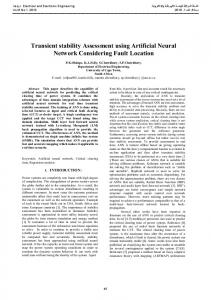
For the scope of this work, a “D”-Shaped two-dimensional bluff body geometry was chosen as a generic wake flow developing a von Kármán vortex street. The geometry is a semi ellipse with an aspect ratio of 35:2. This geometry was chosen to provide room for actuator implementation in future wind tunnel studies. The reference length for the Reynolds and Strouhal numbers is the base height, H. The Reynolds number based on H was Re=300. The wake can be controlled by two blowing and suction slots which are located at the rear corners of the body and are angled at 30 degrees to the free stream direction. A structured, body fitted “D” grid with about 200,000 points is used for the CFD simulation (see Figure 1). This grid is stretched to cluster the grid points tightly in the shear layers of the near wake, as well as around the blowing and suction slots. Uniform flow boundary conditions at the far field are imposed using Riemann invariants. To ensure computational efficiency, the Mach number is set to M=0.1. The time step is ∆t=0.005H/U, where U is the free stream velocity. A previous study by Siegel et al.17 using this grid showed good comparison of the resulting Strouhal number with experimental results. For the purpose of POD model development, the computational results are truncated in space to the bounding box shown in Figure 1. The bounding box extends from 1H upstream of the base, to 9H downstream. In the vertical direction, the flow is truncated to ±2H. This region of interest encloses the vortex formation region entirely; outside of it, the flow is mostly steady. The bounding box contains about 40 000 grid points. 4
y/H
2 0 −2 −4 −10
−8
−6
−4
−2
0 2 x/H
4
6
8
10
Figure 1 Body Geometry, CFD gridpoints and POD bounding box During the simulation, the flow is impulsively started from rest at time t=0s. As a result of the wake instability, the limit cycle oscillation known as the von Kármán vortex street develops. This is shown in Figure 2 where it can be seen that the flow requires about 20 shedding cycles to develop a limit cycle oscillation as witnessed by the lift force. 0.06
13 12 14 11 10
0.04
15 17 19 21 16 18 20
9 8
Lift Force [N]
Downloaded by UNIVERSITY OF CINCINNATI on December 7, 2014 | http://arc.aiaa.org | DOI: 10.2514/6.2007-1166
II.
7
0.02
6 5 1 2 3 4
0 2
Lift Force Segmentation
4
6
0
0.5
1 1.5 2 Simulation Time [s]
2.5
3
Figure 2 Unsteady Lift force during development of limit cycle and SPOD bin segmentation. The goal in modeling this flow field is both in the accurate representation of the flow energy, as well as in deriving spatial modes that capture the physical behavior with one or a pair of modes being attributable to a certain aspect of the main flow behavior, like mean flow, von Kármán vortex shedding modes, and higher order vortex shedding modes. This separation of the flow into individual modes representing physical phenomena is a key requirement for the development of feedback controllers that control these particular flow features. 3 American Institute of Aeronautics and Astronautics
III.
DPOD Procedure
POD techniques are an efficient means to reduce spatially highly complex flow fields by representing them by a small number of spatial modes and their temporal coefficients13. n
u ( x, y, t ) = ∑ ak (t )φk ( x, y )
(1)
Downloaded by UNIVERSITY OF CINCINNATI on December 7, 2014 | http://arc.aiaa.org | DOI: 10.2514/6.2007-1166
k =1
Equation 1 shows this decomposition, where a velocity component or vector u is represented by the spatial modes φk(x,y) and temporal coefficients ak(t) While this decomposition is well suited to time periodic flow fields, it faces problems for transient flows (see Siegel et al.18). Different additions to the basic POD procedure have been proposed, most notably the addition of a shift mode as introduced independently by Noack, Afanasiev, Morzynski and Thiele19 as well as Siegel, Cohen and McLaughlin20. This shift mode originally only addressed changes to the mean flow, but this concept has been extended recently by Siegel, Cohen, Seidel and McLaughlin14 to adjust the fluctuating modes of transient flows as well. This modified POD procedure, referred to as Double POD (DPOD) procedure, provides shift modes for all main modes of a transient flow field. In Equation (2), the index i refers to the main modes of the original POD procedure, while the index j identifies the shift mode order. I
J
u ( x, y, t ) = ∑∑ α ij (t )Φ ij ( x, y ).
(2)
i =1 j =1
Reference is made to all modes with index k>1 as shift modes, since they modify a given main mode (index j=1) to match a new flow state due to transient effects. This may be due to effects of forcing, changes in Reynolds number, feedback or open loop control or similar events. Thus, in the truncated DPOD mode ensemble for each main mode, one or more shift modes may be retained based on inspection of energy content or spatial structure of the mode. For further details on the DPOD procedure refer to Siegel et al.14. Figure 3 shows a DPOD mode set for the transient simulation introduced in Figure 2, retaining 5 main modes and 2 shift modes for each of the five main modes. Modes (1,n) represent the mean flow, Modes (2,n) and (3,n) the von Karman vortex street, while Modes (4,n) and (5,n) represent a higher order vortex shedding mode with twice the spatial frequency of the von Karman vortex street. Inspecting the energy contents of these modes presented in Figure 4, it can be seen that most energy is contained in the mean flow, followed by the von Karman vortex street modes which appear as pairs of approximately equal energy. This behavior is identical to a conventional POD procedure performed on a time periodic flow field. The energy content of the entire mode basis is now a two dimensional energy plane, with steep energy drop-off both towards higher order main and higher order shift modes. While the energy content drop-off of the shift modes of the mean flow mode (Modes (1,2) and (1,3)) is fairly steep, it can be seen that the drop-off for the shift modes of the von Karman modes (Modes (2,2), (2,3) and (3,2), (3,3)) is far less steep, demonstrating the importance of including these modes in a low order model. Since the drop-off in energy is not uniform for all shift modes, one might retain a different number of shift modes for each main mode based on energy considerations. Using this DPOD procedure, accurate transient spatial mode sets have been developed. The next step towards a dynamic model, which represents the temporal behaviour of the unsteady forced wake, is derived from the mode amplitudes obtained from the DPOD procedure. The low dimensional model that represents the time-dependent coefficients of the POD will be derived using a non-linear system identification approach based on artificial neural networks (ANN) as described by Cohen et al21. The DPOD model developed for the transient startup of the vortex shedding behind the D-shaped cylinder was truncated to 5 main and 3 shift modes. The corresponding mode amplitudes are shown in Figure 3, the spatially averaged estimation error in Figure 4. The spatially averaged error is calculated from the averaged difference between the exact velocity flow field and recomposed velocity flow field, which is obtained by multiplying the 15 spatial DPOD modes by their corresponding mode amplitude (see Figure 3). It can be seen that the temporal behavior of the DPOD mode amplitudes is highly nonlinear during the evolution of the limit cycle. However, the average estimation error stabilizes at about 1.25% of the free stream velocity, with higher excursions at the very beginning of the simulation. The goal for feedback control is to be able to estimate the mode amplitudes shown in Figure 4 so that a controller can be developed that acts upon these mode amplitudes. In a typical setup, sensors may be installed on the surface of the model to obtain readings, which are then used to estimate the mode amplitudes by means of linear or nonlinear mapping. 4 American Institute of Aeronautics and Astronautics
1
1
1
0
y/H
2
−1
0
−2
−2 0
2
4
6 x/H
8
10
12
0
2
4
0
12
1
1
0
y/H
1
0
4
6 x/H
8
10
0
12
2
DPOD Mode (3,1)
4
6 x/H
8
10
0
12
1
y/H
1
y/H
1
0
4
6 x/H
8
10
12
0
2
DPOD Mode (4,1)
4
6 x/H
8
10
0
12
1
y/H
1
y/H
1
0
4
6 x/H
8
10
12
0
2
DPOD Mode (5,1)
4
6 x/H
8
10
0
12
1
y/H
1
y/H
1
0
4
6 x/H
8
10
12
10
12
4
6 x/H
8
10
12
10
12
0
−2
−2 2
8
−1
−1
−2
6 x/H
DPOD Mode (5,3) 2
0
2
DPOD Mode (5,2) 2
−1
4
0
2
0
12
−2
−2 2
10
−1
−1
−2
8
DPOD Mode (4,3) 2
0
2
DPOD Mode (4,2) 2
−1
6 x/H
0
2
0
4
−2
−2 2
12
−1
−1
−2
10
DPOD Mode (3,3) 2
0
2
DPOD Mode (3,2) 2
−1
8
0
2
0
6 x/H
−2
−2
2
4
−1
−1
0
2
DPOD Mode (2,3) 2
y/H
y/H
10
2
−2
y/H
8
2
−1
y/H
6 x/H
DPOD Mode (2,2)
DPOD Mode (2,1)
y/H
0 −1
−1
−2
Downloaded by UNIVERSITY OF CINCINNATI on December 7, 2014 | http://arc.aiaa.org | DOI: 10.2514/6.2007-1166
DPOD Mode (1,3)
DPOD Mode (1,2) 2
y/H
y/H
DPOD Mode (1,1) 2
0
2
4
6 x/H
8
10
12
0
2
4
6 x/H
8
Figure 3 DPOD Model of transient start-up data using 5 main POD modes (first index) and 2 shift modes (second index)
In the following, we investigate the ability of a neural network based estimation method to achieve this using velocity signals as input. The best possible outcome is the error presented in Figure 4; realistic numbers of sensors and inaccuracies of the mapping scheme can cause higher errors, and results for different schemes will be presented in the following section. The flow field spatially averaged error has the merit of knowing at once the total error obtained from the combination of all DPOD modes considered.
5 American Institute of Aeronautics and Astronautics
0
10
Mode 1 Mode 2 Mode 3 Mode 4 Mode 5
Mode Energy
Downloaded by UNIVERSITY OF CINCINNATI on December 7, 2014 | http://arc.aiaa.org | DOI: 10.2514/6.2007-1166
−2
10
−4
10
−6
10
1
2
3
4 5 6 Shift Mode Number
7
8
Figure 4 Energy Content of DPOD modes shown in Figure 3
IV.
DPOD Model of “D” Shaped Cylinder
The DPOD model developed for the transient startup of the vortex shedding behind the D-shaped cylinder was truncated to 5 main and 2 shift modes. The corresponding mode amplitudes are shown in Figure 5, the spatially averaged estimation error in Figure 6. The spatially averaged error is calculated from the averaged difference between the exact velocity flow field and recomposed velocity flow field, which is obtained by the multiplying 15 DPOD modes by each corresponding mode amplitude of Figure 3. It can be seen that the temporal behavior of the DPOD mode amplitudes is highly nonlinear during the evolution of the limit cycle. However, the average estimation error stabilizes at about 1.25% of the free stream velocity, with higher excursions at the very beginning of the simulation. The goal for a Reduced Order Model (ROM) is to be able to estimate the mode amplitudes shown in Figure 5 so that a controller can be developed that acts upon these mode amplitudes. In a typical setup, sensors may be installed on the surface of the model to obtain readings, which are then used to estimate the mode amplitudes by means of linear or nonlinear mapping. In the following, we investigate the ability of a neural network based estimation method to achieve this using velocity signals as input. The best possible outcome is the error shown in Figure 4, realistic numbers of sensors and inaccuracies of the mapping scheme can cause higher errors, whose results will be presented in the following section. This flow field spatially averaged error has the merit of knowing at once the total error superposed of all mode amplitudes of DPOD modes.
6 American Institute of Aeronautics and Astronautics
Mode 1,1
Mode 1,2 500
200
−5200
0
0
−5400
−500
−200
−5600 0
2
4
−1000 0
Mode 2,1
2
4
−400 0
Mode 2,2 400
200
500
200
100
0
0
0
−500
−200
−100
−1000 0
2
4
−400 0
Mode 3,1
2
4
−200 0
Mode 3,2 400
200
500
200
100
0
0
0
−500
−200
−100
2
4
−400 0
Mode 4,1 200
200
100
0
0
−200
−100 2
4
−200 0
Mode 5,1 200
200
100
0
0
−200
−100 2
4
−200 0
2
−200 0
4
2
4
Mode 4,3 200 100 0
2
4
−100 0
Mode 5,2
400
−400 0
4
Mode 4,2
400
−400 0
2
4
Mode 3,3
1000
−1000 0
2
Mode 2,3
1000
2
4
Mode 5,3 200 100 0
2
4
−100 0
2
4
Figure 5 DPOD Mode amplitudes 0.03
0.025
Avg Error U/Uinf
Downloaded by UNIVERSITY OF CINCINNATI on December 7, 2014 | http://arc.aiaa.org | DOI: 10.2514/6.2007-1166
Mode 1,3
−5000
0.02
0.015
0.01
0.005 0.5
1
1.5
2 2.5 3 Simulation Time [s]
3.5
4
Figure 6 Flow field spatially averaged error of the 5x3 truncated DPOD model as a function of time 7 American Institute of Aeronautics and Astronautics
Downloaded by UNIVERSITY OF CINCINNATI on December 7, 2014 | http://arc.aiaa.org | DOI: 10.2514/6.2007-1166
V.
Application of ANNE to DPOD Model
The time histories of the mode amplitudes of the DPOD model are determined by mapping the flow field data onto the spatial Eigen functions using one of the estimation techniques described in detail in this section. The intent of the proposed strategy is that the velocity measurements provided by the sensors are processed by the estimator to provide the estimates of the six most energetic modes of the DPOD model. The issue of sensor placement and number has been dealt with in detail by Cohen et al.15 for the case of a circular cylinder and in this effort a similar strategy for determination of the sensor configurations is utilized. Only the stream-wise velocity component was used for the sensor placement and number studies reported in this effort. The main idea in determining the sensor locations is to place the sensors on the extrema of the spatial Eigen functions in the wake as seen in Figure 3 and described in detail by Cohen et al.15 Additionally, a minor sensitivity study was conducted to obtain the final locations and number of the sensors for each of the sensor configurations examined. The locations of the sensors for the two different sensor configurations studied (see Table 1) are referenced in terms of the CFD coordinates (the origin is at the center of the base of the body), non-dimensionalized with respect to the cylinder base height, H, namely, X/H and Y/H. The criterion for quantifying the quality of the prediction is based on the RMS error of the prediction. We define the RMS error as the RMS of the error between the estimated modes based on sensor measurements (using any of the possible estimation techniques, ANNE for example) and the DPOD mode amplitudes obtained form the CFD simulation using the full flow field information. For sake of convenience, this RMS error is normalized with the RMS of the exact mode amplitudes using the full flow field information, presented as a percentage. The resulting error percentage and the number of sensors may be integrated together into a cost function and the purpose of the design process would then be to select the configuration that minimizes this cost. Number of Sensors in Sensor Configuration
4
8
Non-dimensionalized Targeted Mode of each Non-dimensionalized Location of Sensor Location of Sensor sensor X/H Y/H 4.0 0.0 Mode 1,2 1.5 -0.7 Mode 2,1 4.0 -0.8 Mode 3,1 7.0 0.0 Mode 2,2 1.0 0.0 Mode 1,1 4.0 0.0 Mode 1,2 1.5 -0.7 Mode 2,1 4.0 -0.8 Mode 3,1 6.0 0.0 Mode 3,2 7.0 0.0 Mode 2,2 2.5 -0.8 Mode 3,1 6.0 -0.8 Mode 2,1 Table 1: Locations of the sensors in the two sensor configurations studied
Now that the sensor number and location is determined, we develop an estimator based on artificial neural networks (ANN). The decision to look into the ANN class of universal approximators is for their inherent robustness and capability to approximate any non-linear function to any arbitrary degree of accuracy. The ANNE, employed in this effort, in conjunction with the ARX model23-24 is the mechanism with which the dynamic model is developed using the POD mode amplitudes extracted from the high resolution CFD simulation. Non-linear optimization techniques, based on the back propagation method, are used to minimize the difference between the extracted POD mode amplitudes and the ANN while adjusting the weights of the model .22-23 The main hypothesis is that the nonlinearity and scaling characteristics of the temporal coefficients lead to numerical stability issues which undermine the development and analysis of effective estimation/control laws. In order to assure model stability, the ARX dynamic model structure is incorporated. This structure is widely used in the system identification community. A salient feature of the ARX predictor is that it is inherently stable even if the dynamic system to be modeled is unstable. This characteristic of ARX models often lends itself to successful modeling of unstable processes as described by Nelles.22
8 American Institute of Aeronautics and Astronautics
Downloaded by UNIVERSITY OF CINCINNATI on December 7, 2014 | http://arc.aiaa.org | DOI: 10.2514/6.2007-1166
Feature of ANNE Architecture Input Layer
8 Sensor configuration
4 Sensor Configuration
No past outputs; 2 past inputs each No past outputs; 4 past inputs each with 8 time delays i.e. ~ half a with 4 time delays i.e. ~ half a shedding cycle. 129 Neurons (8 x 2 shedding cycle. 65 Neurons (4 x 4 x 4 x 8 +1 bias = 129) in the input layer. +1 bias = 65) in the input layer. Hidden Layer The ANN utilizes just one single hidden layer consisting of 15 neurons. The activation function in the hidden layer is based on the non-linear tanh function. A single bias input has been added to the output from the hidden layer. Output Layer Fifteen outputs, namely, the 15 DPOD states representing the temporal coefficients of the 15 mode DPOD reduced order model developed in Section IV. The output layer has a linear activation function. Weighing Matrices The weighting matrices between the The weighting matrices between the input layer and the hidden layer input layer and the hidden layer (W1) (W1) and between the hidden layer and between the hidden layer and the and the output layer (W2) depend on output layer (W2) depend on the the number of sensors. For example, number of sensors. For example, for for the single sensor case W1 is of the single sensor case W1 is of the the order of [129*15] and W2 is of order of [65*15] and W2 is of the order the order of [16*15]. These of [16*15]. These weighting matrices weighting matrices are initialized are initialized randomly. randomly. Training of the ANN Back propagation, based on the Back propagation, based on the Levenberg-Marquardt algorithm, Levenberg-Marquardt algorithm, was was used to train the ANN using used to train the ANN using Nørgaard Nørgaard et al’s toolbox.23 The et al’s toolbox.23 The training training procedure converged near procedure converged near 200 50 iterations. Of the 341 snapshots, iterations. Of the 341 snapshots, the the first 170 were used for training. first 170 were used for training. Validation of the ANN Of the 341 snapshots, the final 171 snapshots were used for validation purposes. RMS Errors for the validation data set is shown in Table 3 Table 2 Details of the ANNE Architecture and Design used for the two Sensor Configurations In this effort, the method of choice is based on a nonlinear system identification approach described by Nelles22 using Artificial Neural Networks (ANN) and ARX models23-24. For the application of the multilayer perception to the multi input and multi output system, the integrated ANN/ARX forms the basis for the algorithm used in ANNE. First, based on an adequate training set, the ANN network is designed and then with new data the “frozen” ANN design, with its associated weighing matrices, is validated. The purpose is to obtain a robust and real-time estimator for as low a number of sensors as possible for application to the wake control. For the mapping of velocity measurements provided by the sensors onto the mode amplitudes of the fifteen DPOD modes, the modified NNARXM20 (Neural Network Autoregressive, eXternal input, Multi output) algorithm, originally developed by Nørgaard et al,23 is used as ANNE (Artificial Neural Network Estimation) because of its inherent robustness and capability to approximate any non-linear function to any arbitrary degree of accuracy. For each sensor configuration, 341 velocity measurements, equally spaced at 0.01 seconds apart, were used. Of the 341 snapshots, the first 170 were used for training of the estimator, whereas the final 171 snapshots were used for validation purposes. For the Multilayer Perceptron Neural Network, the NNARXM is chosen as an ANNE. The artificial neural network (ANN) has the salient features detailed in Table 2.
9 American Institute of Aeronautics and Astronautics
Downloaded by UNIVERSITY OF CINCINNATI on December 7, 2014 | http://arc.aiaa.org | DOI: 10.2514/6.2007-1166
The results using ANNE is presented in Table 3 for each of the two sensor configurations in terms of the nondimensionalized RMS error (presented as a percentage). These results, with respect to the RMS error, compare very well to those presented using Linear Stochastic Estimator (LSE), developed by Adrian25, for the identical 8 sensor configuration (see Figure 7). Furthermore, we would like to quantitatively examine the main contributors to this improvement of performance, namely: Nonlinearity vs. linearity; dynamic mapping (“delay” or memory) vs. static mapping; and robustness to noise. The estimation scheme, ANNE, will be compared to other non-linear techniques such as the quadratic stochastic estimation, QSE, proposed by Murray and Ukeiley26 as well as by Ausseur et al.27 as well as introduction of time delays to the LSE, DSE, as examined by Debiasi et al.28 (see Figure 8).
DPOD
ANNE
LSE
ANNE
LSE
DSE
QSE
Modes
8 Sensors
8 Sensors
4 Sensors
4 Sensors
4 Sensors
4 Sensors
1,1
0.04
3.30
0.17
6.84
2.32
1.09
2,1
0.38
12.96
2.40
33.63
8.48
20.54
3,1
0.22
29.04
1.49
84.54
7.43
57.05
1,2
1.58
51.85
5.26
53.66
8.99
27.29
2,2
3.87
52.22
11.40
81.06
59.82
44.54
3,2
2.81
89.17
23.60
92.13
65.12
80.31
Table 3 RMS of the Prediction Errors for six DPOD modes [%] Recent work by Cohen et al.21 shows that effective suppression of the cylinder wake is possible with feedback based on the first periodic DPOD mode, Mode 2,1 and the shift mode, Mode 2,2. We believe that effective feedback should be possible using the first three modes and their associated shift modes. For this comparative study between four different estimation techniques, the four sensor case is examined. These techniques are as follows: • Linear Stochastic Estimation (LSE) which forms a baseline, based on the approach developed by Adrian25. • Quadratic Stochastic Estimation (QSE) which includes quadratic terms, based on the quadratic stochastic estimation proposed by Murray and Ukeiley26 as well as by Ausseur et al.27. • Dynamic Stochastic Estimation (DSE) which includes 3 time delays as additional inputs to that at time t (in all 4 input signals per sensor) along the lines examined by Debiasi et al. for the cavity acoustic suppression problem28. • Artificial Neural Network Estimation (ANNE) as developed in this paper.
Linear Terms
LSE
QSE
DSE
ANNE
Si(t)
Si(t)
Si(t)
Si(t)
-
-
Si(t-1), Si(t-2), Si(t-3)
Si(t-1), Si(t-2), Si(t-3)
Quadratic Terms
-
Time Delay Terms
-
“Auto” Terms: Si2(t), “Cross” Terms: S1S2(t), S1S3(t), S1S4(t) S2S3(t) S2S4(t) S3S4(t) -
Total Number of Signal Inputs to 4 14 16 16 Estimation Scheme Table 4. Description of the information required for each of these estimation techniques. The number of sensors is i=1,2,3,4.
10 American Institute of Aeronautics and Astronautics
Downloaded by UNIVERSITY OF CINCINNATI on December 7, 2014 | http://arc.aiaa.org | DOI: 10.2514/6.2007-1166
Figure 7 Mode amplitudes aij of the 6 DPOD modes for the validation data set based on the 8 sensor configuration. This data was not used for training of the estimators. Black Lines, mode amplitudes from the CFD simulation. Blue symbols, mode amplitude estimation from the ANNE model. Red symbols, mode amplitudes obtained using LSE.
11 American Institute of Aeronautics and Astronautics
Downloaded by UNIVERSITY OF CINCINNATI on December 7, 2014 | http://arc.aiaa.org | DOI: 10.2514/6.2007-1166
Figure 8 Mode amplitudes aij of the first 6 DPOD modes for the validation data set based on the 4 sensor configuration. This data was not used for training of the estimators. Black Lines, mode amplitudes from the CFD simulation. Blue symbols, mode amplitude estimation from the ANNE model, whereas the red symbols are the mode amplitudes obtained using LSE. The green symbols depict DSE predictions and the magenta colored symbols illustrate QSE predictions.
12 American Institute of Aeronautics and Astronautics
Downloaded by UNIVERSITY OF CINCINNATI on December 7, 2014 | http://arc.aiaa.org | DOI: 10.2514/6.2007-1166
In Table 4, the information required for each of these estimation techniques is presented. We can clearly see that for the baseline LSE case only instantaneous linear terms are required. The other schemes require more information which includes quadratic terms or time delays. The DSE and ANNE require exactly the same amount of information. The results for the four estimation techniques are presented in Table 3 and the following observations can be made: • Not surprisingly, ANNE provides superior results for the 8 sensor configuration in comparison to the 4 sensor configuration. The more sensors the better the prediction. However, if we compare the results between the LSE having eight sensors and ANNE with four sensors, we can correlate the performance enhancement with the salient features of the technique, namely, non-linearity and dynamic memory. • There are three parameters one would like to observe in a good prediction and we mentioned one of those being the RMS error. Additionally, for the periodic modes, such as the von Karman shedding modes, Modes 2,1 and 3,1, we would also need to consider the frequency and phase prediction as well. It is interesting to note that both frequency and phase are relatively well predicted by all the four techniques. The main differences are in the amplitude predictions of the four different techniques, which are important when considering feedback control. • The RMS error provided by LSE is significantly improved upon by each of the other three techniques. • ANNE, which uses inputs identical to DSE, provides the best results. This may be attributed to both the inclusion of the time delays as well as the nonlinearities.
VI. Conclusions & Recommendations We introduce Double Proper Orthogonal Decomposition (DPOD) as a means to derive POD spatial modes that span different flow conditions. We demonstrate its ability by applying it to a transient simulation of the development of the limit cycle of a D shaped cylinder wake. Based on a previously validated sensor placement study (Cohen et al.15), a comparison was made between the effectiveness of the conventional LSE versus the newly proposed ANNE for real-time estimation of the low-dimensional POD states based on a few flow field velocity measurements. The development of the procedure used CFD simulation data of a “D” shaped cylinder wake at a Reynolds number of Re=300. For the estimation of the first six DPOD modes, we show that a four sensor configuration using ANNE provides better results than an 8 sensor configuration using the state-of-the-art LSE. We attribute the augmented performance exhibited by ANNE to both its non-linear modeling capability as well as the dynamic behavior due to the inclusion of the time lag terms. This is demonstrated by comparing ANNE to three other techniques, namely, LSE, QSE and DSE, which are being proposed by other researchers in the field. Further research will aim at examining the robustness of the newly proposed ANNE for a situation when the body experiences transient forcing as a result of feedback control. The sensitivity of the number and location of sensors to transient dynamics of the forced cylinder wake needs to be examined before any useful recommendations can be made. Furthermore, for the case of transient forcing, we will systematically and quantitatively reexamine the main contributors to this betterment of performance, namely: nonlinearity vs. linearity; dynamic mapping (“delay” or memory) vs. static mapping; and robustness to noise. In addition, we intend to examine the generic nature of the developed strategy (ANNE) for surface mounted sensor configurations based on pressure or skin friction measurements. Finally, we would like to examine the sensitivity of the ANN architecture to performance vs. computational cost for all the above cases.
Acknowledgments The authors would like to acknowledge the support and assistance provided by Lt. Col. Scott Wells (AFOSR) and Dr. James Myatt (AFRL). The authors would like to thank Dr. Jim Forsythe for providing the CFD grid.
References 1
Gillies E A., “Low-dimensional Control of the Circular Cylinder Wake”, Journal of Fluid Mechanics, 1998, Vol. 371, pp. 157-78. 2 von Kármán T, Aerodynamics: Selected Topics in Light of their Historic Development, New York: Cornell University Press, Ithaca, 1954.
13 American Institute of Aeronautics and Astronautics
Downloaded by UNIVERSITY OF CINCINNATI on December 7, 2014 | http://arc.aiaa.org | DOI: 10.2514/6.2007-1166
3 Park DS, Ladd DM, and Hendricks EW, “Feedback Control of a Global Mode in Spatially Developing Flows”, Physics Letters A, 1993, Vol. 182, pp.244-248. 4 Roussopoulos K., “Feedback Control of Vortex Shedding at Low Reynolds Numbers”, Journal of Fluid Mechanics, 1993, Vol. 248, pp.267-296. 5 Cohen, K., Siegel, S., and McLaughlin, T, "Control Issues in reduced-Order Feedback Flow Control", Invited Lecture at session titled "Closed-Loop Flow Control: Algorithms and Applications", AIAA Paper 2004-0575, 42nd AIAA Aerospace Sciences Meeting, Reno, Nevada, January 5-8 2004. 6 Noack, B.R., Tadmor, G., and Morzynski, M., "Actuation models and dissipative control in empirical Galerkin models of fluid flows", 2004 American Control Conference, June 30 - July 2, 2004 at the Boston Sheraton Hotel in Boston, MA, Paper FrP15.6. 7 Noack, B.R., Tadmor, G., and Morzynski, M., "Low-dimensional models for feedback flow control. Part I: Empirical Galerkin models", 2nd AIAA Flow Control Conference, 28 Jun - 1 Jul 2004, Portland, Oregon, AIAA-2004-2408. 8 Tadmor, G., Noack, B.R., Morzynski, M., and Siegel, S., "Low-dimensional models for feedback flow control. Part II: Observer and controller design", 2nd AIAA Flow Control Conference, 28 Jun - 1 Jul 2004, Portland, Oregon, AIAA Paper 20042409. 9 Glauser, M., Higuchi, H., Ausseur, J., Pinier, J., "Feedback Control of Separated Flows (Invited)", 2nd AIAA Flow Control Conference, 28 Jun - 1 Jul 2004, Portland, Oregon, AIAA Paper 2004-2521. 10 Yuan, X., Caraballo, E., Yan, P., Özbay, H., Serrani, A., DeBonis, J., Myatt, J., and Samimy, M., "Reduced-order Modelbased Feedback Controller Design for Subsonic Cavity Flows", 43rd AIAA Aerospace Sciences Meeting, Reno, Jan. 10-13 2005, AIAA Paper 2005-0293. 11 Luchtenburg, M., B. Noack and R. King, G. Tadmor, “Tuned POD Galerkin Models for Transient Feedback Regulation of the Cylinder Wake”, AIAA-2006-1407, 44th AIAA Aerospace Sciences Meeting and Exhibit, Reno, NV, January 2006. 12 Stalnov, O., Palei, V., Fono, I., Cohen, K., and Seifert, A., "Experimental Validation of Sensor Placement for Control of a "D" Shaped Cylinder Wake", AIAA-2005-5260, 35th AIAA Fluid Dynamics Conference and Exhibit, Toronto, Canada, June 6-9, 2005. 13 Holmes, P., Lumley, J.L., Berkooz, G., Turbulence, Coherent Structures, Dynamical Systems and Symmetry, Cambridge University Press, Cambridge, 1996. Chap. 3. 14 Siegel S., Cohen K., Seidel, J., and McLaughlin T, “State estimation of transient flow fields using Double Proper Orthogonal Decomposition (DPOD)”, International Conference on Active Flow Control, Berlin, Germany, September 27-29, 2006. 15 Cohen, K., Siegel, S., and McLaughlin, T.,"A Heuristic Approach to Effective Sensor Placement for Modeling of a Cylinder Wake”, Computers & Fluids, Vol. 35, Issue 1 , January 2006, pp. 103-120. 16 Shin, Young-Sug, Cohen, K., Siegel, S., Seidel, J., and McLaughlin, T., “Neural Network Estimator for Closed-Loop Control of a Cylinder Wake”, AIAA Guidance, Navigation, and Control Conference and Exhibit, Keystone, Colorado, 21 - 24 Aug 2006, AIAA-2006-6428. 17 Siegel, S., Cohen, K., Seidel, J., and McLaughlin, T., “Two Dimensional Simulations of a Feedback Controlled D-Cylinder Wake”, AIAA Fluid Dynamics Conf Toronto, ON, CA, AIAA 2005-5019, 2005. 18 Siegel, S., Cohen, K., Seidel, J., McLaughlin, T., 'Short Time Proper Orthogonal Decomposition for State Estimation of Transient Flow Fields', 43rd AIAA Aerospace Sciences Meeting, Reno, AIAA2005-0296, 2005. 19 Noack, B.R., Afanasiev, K., Morzynski, M., and Thiele, F., “A hierarchy of low dimensional models for the transient and post-transient cylinder wake”, J. Fluid Mechanics, vol. 497, pp. 335–363, 2003. 20 Siegel, S. Cohen, K., and McLaughlin., T., "Numerical simulations of a feedback controlled circular cylinder wake", AIAA Journal, vol. 44, no. 6, pp.1266-1276, June 2006. 21 Cohen, K., Siegel, S., Seidel, J., and McLaughlin, T., “Low dimensional modeling, estimation and control of a cylinder wake”, Invited lecture at Session "Order Reduction and Control for Aerodynamics", 45th IEEE Conference on Decision and Control, San Diego, 13-15 December 2006. 22 Nelles, O., Nonlinear System Identification, Springer-Verlag, Berlin, Germany, 2001, Chap. 11. 23 Nørgaard, M., Ravn., O., Poulsen, N.K., and Hansen, L.K., Neural Networks for Modeling and Control of Dynamic Systems, 3rd printing, Springer-Verlag, London, U.K., 2003, Chap. 2. 24 Ljung, L., System Identification: Theory for the User, 2nd Edition, Prentice Hall, Upper Saddle, NJ, USA, 1999, Chap.4. 25 Adrian, R.J., “On the Role of Conditional Averages in Turbulence Theory”, In Proceedings of the Fourth Biennial Symposium on Turbulence in Liquids, J. Zakin and G. Patterson (Eds.), Science Press, Princeton, 1977. 26 Murray, N.E., and Ukeiley, L.S., “Estimating the Shear Layer Velocity Field Above an Open Cavity from Surface Pressure Measurements”, 32nd Fluid Dynamics Conference and Exhibit, 24-26 June 2002, St. Louis, MO, AIAA Paper 2002-2866. 27 Ausseur, J. M., Pinier J., T., Glauser, M.N., Higuchi H., and Carlson, H., “Experimental Development of a Reduced-Order Model for Flow Separation Control”, 44th AIAA Aerospace Meeting and Exhibit, 9-12 January 2006, Reno, Nevada, AIAA Paper 2006-1251. 28 Debiasi, M., Little, J, Caraballo, E., Yuan, X., Serrani, A., Myatt, J.H., and Samimy, M., “Influence of Stochastic Estimation on the Control of Subsonic Cavity Flow – A Preliminary Study”, 3rd AIAA Flow Control Conference, San Francisco, California, 5 - 8 June 2006, AIAA-2006-3492.
14 American Institute of Aeronautics and Astronautics