Evolutionary Algorithm Use in Optimisation of a Launch Vehicle Stack ...

AIAA 2007-364

45th AIAA Aerospace Sciences Meeting and Exhibit 8 - 11 January 2007, Reno, Nevada

Evolutionary Algorithm use in Optimisation of a Launch Vehicle Stack Model G.P.Briggs, Tapabrata Ray & J.F.Milthorpe. School of Aeronautical, Civil and Mechanical Engineering, University of New South Wales at Australian Defence Force Academy, Northcott Drive, Canberra, ACT 2600, Australia

Conceptual design of a satellite launch vehicle is a multidisciplinary task which must take into account interactions of discipl ines such as propulsion, aerodynamics, structures, guidance and orbital mechanics. We discuss the initial modeling of a clean sheet design for a satellite launch vehicle capable of placing an Ariane-44L equivalent payload into geostationary transfer orbit. The proposed vehicle is a straight three stage vehicle as distinct from AR44L which was a three and a half stage vehicle. The Delta-V capability or “ideal -velocity” of the AR44L is first derived from published data then the proposed design is modelled using a spreadsheet. The Gross Lift-Off Weight of the vehicle is then minimised for the same delta-V as Ariane. Various differences between the two vehicles are discussed. The initial design of an SLV as presented is based on a simple stack model optimised automatically using an evolutionary algorithm. The efficiency of the proposed approach is discussed along with future developments in the areas of vehicle model and multiobjective formulations of the design optimisation problem.

I.

Introduction

O

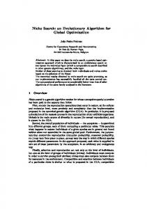
ur interest at the School of Aerospace, Civil and Mechanical Engineering (ACME) is to develop a framework that supports multidisciplinary conceptual design of expendable satellite launch vehicles. For a start, a simple stack model of the launch vehicle was considered to understand the behavior of the optimisation algorithms and problem formulations. The final aim being the ability to optimise designs using a detailed model of a launch vehicle including optimised trajectory, structure and engine design parameters. This simple model was sufficiently valid to be able to give first order vehicle mass estimates to be input into the more detailed program. It was also used to give students a feel for the initial sizing of a launch vehicle. As a first step towards the more detailed model, the Gross Lift-Off Weight (GLOW) of the vehicle was required to be minimised on the initial assumption that the lowest cost vehicle corresponded to the lightest weight vehicle. Evolutionary optimisation techniques were used to choose masses of the three stages that would minimise the GLOW. A number of other parameters, as described below, were assumed constant and were not optimised. It was initially desired to model a clean-sheet design for a three stage launch vehicle with payload and much of the design equivalent to the Ariane 44L (AR44L) vehicle . While the AR44L design is a three and a half stage vehicle due to four liquid fuel strap-on boosters being staged in parallel with the main first stage of the vehicle, the proposed HLV (Hypothetical Launch Vehicle) design was to be a straight three stage vehicle (Figure 1). The questions to be answered were, how much heavier would this design be than that of AR44L, how the evolutionary Figure 1 . Diagram of Ariane 44L & HLV 1 American Institute of Aeronautics and Astronautics

Copyright © 2007 by Gordon P Briggs, Tapabrata Ray, John F Milthorpe. Published by the American Institute of Aeronautics and Astronautics, Inc., with permission.

methods would perform in determining a minimum GLOW and how sensitive would the results be. In addition, the model was required to be able to be used to design other proposed launch vehicles moving away from the AR44L design parameters .

II.

Method

In order to obtain realistic mass and delta-V values for the model, the Ariane 44L was used as a baseline against which to compare results from the model. Analysis of the performance capability of AR44L was carried out by applying the rocket equation to each stage and obtaining the ideal velocity of the entire vehicle. The delta-V of the AR44L was determined to be 11794.1 m/sec and the delta-V required from the hypothetical three stage vehicle (HLV) was the same as that of the Ariane vehicle. While quoted masses of AR44L components vary from reference to reference the masses used were the best available from easily obtainable sources priumarily the Ariane User’s Manual1, along with specific impulse performance and structure factor data for each stage from the same source. Identical payload and accommodation masses were used Table 1. Payload and equipment masses used for the HLV model as exist in the AR44L vehicle and are for both AR44L and HLV models shown in Table 1. The HLV was initially modelled on an MSItem Mass, kg Excel spreadsheet program (STAGEX) and in parallel, a Fairing 900 FORTRAN program (ROKOPT) was written to duplicate Payload 4768 those results . ROKOPT was to be the basis of a full launch Adapter 200 vehicle model and it was used here to test the evolutionary Vehicle Equipment Bay 400 optimisation methods to be used later on the full model. A. Spreadsheet Method The initial methodology involved displaying the HLV stack mass breakdown on an MS-Excel spreadsheet (STAGEX) and carrying out an optimisation to maximise the delta-V delivered by the stack. The prop ellant specific impulses and the stage structure factors were assumed to be identical to the AR44L vehicle. Implicit in this scenario is the assumption that the propellant combinations used in the two vehicles are also identical. In reality identical structure factors are not likely to occur because of the greatly differing sizes of the stages of the two vehicles. The AR44L analysis above includes an allowance of 200kg for third stage contingency or margin propellant. This estimate is based on hearsay only as the actual figure could not be determined. This amounts to ~1.7% of the third stage propellant and is the percentage that is allowed in the HLV even though the third stages of the two vehicles differ greatly in size. In addition the Ariane payload fairing is jettisoned during the second stage burn at a height that depends on the aerothemal flux that can be tolerated by the payload. This can make a difference of up to 14kg in payload and a variation of 14 seconds in the mission time of fairing jettison. In the HLV we consider the fairing to be always jettisoned just before or at second stage burnout. Initial stage masses, including propellant, chosen by any of a number of Table 2. Optimal stage masses for methods (including guessing) were entered into the spreadsheet and modified HLV as determined by STAGEX until the desired delta-V was obtained. The initial stack was modified by HLV Stage Stage Mass, entering mass exchange values into dedicated cells to investigate the effect on kg the delta-V of moving mass from one stage to another. Once the delta-V was 3 29700 maximised the whole vehicle was resized to once again give the target delta-V. 2 91600 The process was repeated until minimum GLOW was achieved. 1 346200 This method illustrates the optimisation of a launch vehicle stack with a single objective function (GLOW) and a single constraint to be observed GLOW 473800 (delta-V). The results of the manual spreadsheet optimisation gave a GLOW Delta-V 11794.1 of 473800 kg for the target delta-V of 11794.1 m/sec, which is about m/sec 6 tonnes lighter than the AR44L. The resultant stage masses are shown in Table 2. The result of the STAGEX optimisation shows that as a consequence of effectively reducing the size of the first stage by eliminating the four liquid strap-on boosters the HLV vehicle requires that its two upper stages be considerably larger than those of AR44L while the first stage is about 81% the mass of the combined AR44L first stage and strap on boosters .

2 American Institute of Aeronautics and Astronautics

B. Velocity Budget The equations for launch vehicle sizing are well known and can be found in many texts . For example, White2 develops the equations for single, multiple and infinite numbers of stages with like and unlike stage parameters. There is however no analytical method which allows the equations describing a multistage launch vehicle to be solved for the optimum mass ratios of each stage if the effects of drag and gravity are considered3. Vehicle design is dependent on the delta-V to be achieved which is partly dependent on the trajectory flown, which in turn is dependent on the vehicle design. There is therefore no closed form solution to the problem. However, If the velocity requirement (or budget) is known, a preliminary launch vehicle design can then be produced to provide the required delta-V. Approximations to the velocity budget to be flown can be made including allowances for thrustatmospheric loss, drag loss, gravity loss, earth rotation gain and orbital velocity required. C. Full Launch Vehicle Model The STAGEX spreadsheet described above was developed to assist with estimating the velocity budget. While the estimates are not exact, they are sufficient to allow an estimate of the stage sizes to be made for use as inputs to a more detailed optimising computer model which will eventually include integration of the trajectory to give guidance parameters and the flight profile. Engine nozzle expansion ratio, thrust atmospheric loss effects , drag, the effects of mixture ratio on the delivered specific impulse, propellant density and hence the structure mass are also to be included. These further developments of the model will include many more variables to be optimised than the simple stack model. It will then not be possible to optimise the variables manually as was done with the STAGEX spreadsheet so an automatic method must be found . In order to test optimisation methods for the full computer model (ROKOPT), a project was set up to run on a Pentium-4 desktop computer under the Windows-XP operating system. The development environment used was MS-Visual Studio with an integrated Compaq Visual Fortran 6.6C compiler. Mixed language projects are supported in this environment so that although the main code was written in Fortran-77 with Fortran 90/95 extension, C++ subroutines could also be automatically compiled and linked within the project . The initial part of the project was to calculate the stack GLOW and delta-V using the data from the HLV vehicle as approximated by the STAGEX spreadsheet. Optimisation code was then added to choose stage masses to minimise the GLOW and constrain the HLV delta-V to the AR44L ideal-velocity. D. Evolutionary Method These optimisation methods rely on the generation of an initial random population of solutions to the problem in which the variables are randomly chosen from a given range near the optimum values. The function is then evaluated for each of the sets of generated variables (designs). The algorithm then generates a child population (set of designs) and better solutions among the set of parents and the child population survive to the next generation observed. After a number of generations the population will converge towards an optimum design. In the case involving the launch vehicle stack, the variables are the stage masses with specific impulse and structure factor as constants. The objective function is minimum GLOW and the constraints to be observed are the upper and lower delta-V velocity values . Populations of random values of stage masses lying within the allowed mass ranges are generated then the GLOW is evaluated and the delta -V determined for each set. The delta-V values may not be within the allowed tolerance for the initial generation and can take on any values corresponding to that given by the randomly selected values of the variables. As the generations go by the evolution rules soon move the variable sets into regions where the delta-V constraint is met. The evolutionary optimisation method used in this study is described in detail in Ray and Sarker4. The evolutionary algorithm as develo ped by Ray and Sarker is a variant of NSGA-II 5, 6 with a modified method of population reduction which insists on maintaining the diversity of solutions both in the objective and the variable space. The method is computationally more expensive than NSGA-II but maintains the diversity of the variable space more effectively than NSGA -II.

III.

The Calculations

The problem was to test the optimisation algorithm to determine the number of members of the population and the number of generations required in the evolutionary computation method to obtain a minimum GLOW with the stack delta-V constrained to 11794.1 m/sec. The calculation of the stack mass and Delta-V delivered was coded to include the payload configuration of Table 1, the 1.7% 3rd stage margin propellant and the fairing drop at 2nd stage burnout. While the Delta-V target represents one physical constraint, the minimisation routine was given two constraints, viz., delta-V+e and delta-V-e, 3 American Institute of Aeronautics and Astronautics

where e is the residual allowed in the delta-V at convergence. The routines were therefore working with three variables (viz., the three stage masses), one objective function t o be minimised (GLOW) and two constraints to be observed. While an acceptable residual was deemed to be 0.1 m/sec, in Table 3. Stage mass ranges for the HLV as all calculations e was set to be 0.01 m/sec as it was found that the input to ROKOPT Run-A constraint was quickly reached during the optimisation with the HLV Stage Stage Mass Range, kg minimum GLOW taking longer to be found. In the first test the 3 26800 – 32900 initial stage size estimates were derived from STAGEX and the 2 83400 – 102000 ranges used allowed for an approximately ±10% spread of 1 316000 - 386500 input solutions to the problem (Table 3). GLOW To be minimised The random number generator used to generate the random Delta-V 11794.1 m/sec solutions for this method was RAN0 following the method of Park and Miller as described in reference 7 A run of 64 optimisations was carried out using all the Table 4. Values of evolutionary parameters used to combinations of the values of the evolution parameters evaluate the stage masses – Run-A shown in Table 4. The number of input solutions Parameter Values generated was 30 as it is normally estimated that 10N should be used where N is the number of variables (viz: the No of solutions 30 three stage masses). Initial test runs demonstrated that 50 full generations (parent and child) were more than Max number of generations 50 sufficient for convergence. Random Seed 0.2, 0.3, 0.4, 0.5 The 64 runs were completed in 37.4 seconds on the Pentium 4: a run time of 0.58 seconds per optimisation. The Probability of crossover 0.90, 0.92 values of the stage masses found for the optimum GLOW of Probability of mutation 0.05, 0.07 each run are listed in Table 5. The minimum values of Distribution index crossover 10, 15 GLOW found for the vehicle vary by approx 1100kg. While the minimum value reported is 67 kg above that obtained by Distribution index mutation 10, 15 the manual optimisation using STAGEX. The first stage masses found vary by 904kg (~0.3%), the second stage masses by 359kg (~3.8%) and for the third stage by 2862kg (~9.6%). While the minimum GLOW found is acceptable, being only 21kg above the STAGEX optimum solution, the range of stage masses is not. A first stage design could not, for instance, be based on a mass uncertain by 2. 3 tonnes. In order to visualise the Table 5. Stage masses for the HLV as determined by ROKOPT Run-A distribution of the values of the optimal solutions found, the Vehicle 1st stage 2 nd stage 3 rd stage GLOW, GLOWs were plotted in mass, kg mass, kg mass, kg kg ascending order (Figure 2). Maximum GLOW 344844 97472 26845 475430 The plot demonstrates straight Minimum GLOW 343940 93874 29707 473789 line segments in the Spread of values 904 3598 -2862 1641 distribution of members of the optimal GLOW solutions. Percentage spread 0.26% 3.83% 9.63% 0.35% Figure 3 shows the optimal Mean Solution 344746 92925 30482 480739 stage masses plotted against Median Solution 343228 93641 30864 474418 their optimal GLOW found. STAGEX Solution 346200 91600 29700 473768 For values of GLOW greater than the minimum there are STAGEX residuals -2260 2274 7 21 several combinations of stage mass values that give the GLOW value. As the GLOW approaches the minimum value towards the left of the graph the range of stage mass values decreases but still does not reach a single optimal solution. It is thus not apparent whether the method has not yet found the minimum or whether there are a number of minimal solutions. Examination of the plots for the first and second stage solutions would in fact indicate that there may be two distinct branches to the plot at lower GLOW values . In order to test the hypothesis that the evolutionary algorithm had not found the minimum GLOW a program run (Run-B) with a mu ch larger number of optimisations was carried out. Table 6 shows the optimisation parameters used for this larger run this time using a population of 100 generated solutions . Once again, 50 generations was sufficient for each optimisation run to converge.

4 American Institute of Aeronautics and Astronautics

Figure 2. Members of the GLOW population of Run-A demonstrating straight line segments in the distribution of values. This corresponded to a total of 1539 optimisation runs and took a total elapsed time of 3495.3 seconds on the Pentium-4 computer. Figure 4 shows that this time the distribution of optimal solutions is not linear but demonstrates some members at extreme high GLOW values . Table 8 shows the maximum and minimum optimal GLOW solutions found by Run-B. The minimum optimal vehicle is now 17kg lighter than the solution found by STAGEX so we conclude that Run-A had not found the minimum optimal solution. The spreads of the stage masses found is still large but this is due to the large number of high GLOW solutions in the population of 1539 runs. The last row in the table presents the difference between the STAGEX solution and the minimum solution found by ROKOPT in Run-B. The residuals are now much smaller than for Run-A. Confirmation that Run-B is reaching a minimum solution can be obtained by examining Figure 5 which is Figure 3. Stage mass solutions against their GLOW the equivalent plot for Run-B as Figure 3 was for solutions – Run-A Run-A. It can be seen that at the lower GLOW values the spread of stage mass values is lower and eventually at the extreme left side of the plot the spread reduces to almost zero. The stage mass residuals with respect to the STAGEX solution (Table 7) have reduced to the several hundred kilogra m level and the ROKOPT solution is better than that of STAGEX by 15 kg. The STAGEX operator gave up trying to find the absolute Table 6. Values of evolutionary parameters used to minimum GLOW at the 0.1 tonne level. We can now assume evaluate the stage masses – Run-B that the evolutionary methods used by ROKOPT have found Parameter Values the absolute minimum to within that level and presumably to No of solutions 100 the order of 15 kg. Examining Table 7, we can see that as the first and second stage masses differ from the STAGEX Max no of generations 50 solution by the order of three to four hundred kilograms, it is Random Seed 0.05, 0.1, … , 0.95 possible to still have a near optimal launch vehicle and not have the stage masses of the absolute optimal vehicle. This Probability of crossover 0.90, 0.92, 0.94 could be useful if in the detailed design of one stage the mass Probability of mutation 0.05, 0.07, 0.09 overruns the desired figure, but only if the overrun can be compensated in the other stages. Choosing an off-optimal Dis tribution index crossover 10, 15, 20 solution may thus be more robust than insisting on an absolute Distribution index mutation 10, 15, 20 minimum solution.

5 American Institute of Aeronautics and Astronautics

Table 7. S tage masses for the HLV determined by ROKOPT Run-B

It is also apparent from Figure 5 that the solutions are Vehicle 1st stage 2 nd stage 3 rd stage GLOW, bounded by an envelope. The mass, kg mass, kg mass, kg kg exact nature of the envelope Maximum GLOW 353001 83555 32860 475684 will be discussed later. What Minimum GLOW 345814 91907 29765 473753 can be said now is that feasible solutions appear inside the Spread of values 7188 8352 3095 1931 envelope and solutions occurring Percentage spread 2.08% 9.09% 10.40% 0.41% outside the envelope are Mean Solution 345436 92466 29980 474149 unfeasible and do not appear. Median Solution 345508 92613 29917 474073 Starting each optimisation with a larger number of STAGEX Solution 346200 91600 29700 473768 members of the initial STAGEX residual -386 307 65 -15 population does not seem to assist in finding the minimum solution as the move from 30 members in Run-A to 100 members in Run-B has not meant that there are no high GLOW values in the solutions. This has yet to be confirmed by further experimentation. What does seem to be the main contributor to finding the local minimum solution is increasing the number of runs each with differing evolutionary parameters.

Figure 4. Members of the GLOW population of Run-B demonstrating several points at high values. This does not mean however that either the STAGEX or ROKOPT solutions have reached the absolute local minimum value of GLOW. The optimisation using STAGEX became difficult around the minimum as the solution wandered around the basin of the local minimum It was not obvious to the operator which way to move the solution to reach the absolute minimum. The evolutionary method on the other hand will eventually choose a minimum and given enough time will automatically do better than STAGEX. A. Specifying the Constraints: In both the ROKOPT runs discussed above the single constraint was the requirement for the vehicle ideal-velocity to be equal to that of Ariane-44L, viz. the calculated value of 11794.1 m/sec. In order to achieve this physical constraint the algorithm was given two numerical constraints, an upper and a lower value to limit the velocity to the band between the two values. Subsequently another method was tried. It was reasoned that because the velocity Figure 5. Stage mass solutions against their GLOW achieved (with a given payload) was dependent on the size of solutions – Run B the launch vehicle, it would be possible to constrain the 6 American Institute of Aeronautics and Astronautics

velocity with one constraint only, namely that the velocity be greater than the required value. With the objective function being the minimisation of the launch vehicle lift off weight the velocity would automatically be decreased until it equaled the constraint value. Test runs showed that this indeed produced the required result. However it was realised that this would only be true if the constraint variable was a direct function of the objective function. Otherwise a range would need to be specified to the algorithm for the value of the constraint unless it was not of concern as to the exact value of the constraint variable except that it was required to be greater or less than a given value (inequality). Imposing an equality requirement such that the constraint variable should be exactly equal to the required value would be too stringent a test as all members of the initial population would then be found to be infeasible. B. Gradient Methods to Supplement the Evolutionary Methods: At the bottom of the basin of the minimum of the objective function it is difficult to find the absolute minimum. This was evident when using the STAGEX spreadsheet as the operator couldn’t determine the best direction to move to find an improvement in the objective. A commercial solver add-in routine for STAGEX (Excel spreadsheet) was obtained to automatically optimise the stack model. The solver routine used an evolutionary method to find the approximate solution and then utilised a gradient method to find the minimum of the basin. Happily, the results obtained using this software agreed exactly with the results obtained using the ROKOPT program thus verifying the ROKOPT results. As a second test a Nelder and Mead8, 9 (NM) multi-dimensional point improvement simplex method (Amoeba) was included in ROKOPT and tested on this problem. It was necessary to implement a penalty function to be able to specify constraints in NM as they are not integral to this method. When using NM it was found that similarly to the EA method, the solutions found depended on the random starting point chosen. This should not be the case for NM and seems to indicate that the introduction of penalty functions which come into play at the constraint boundary is responsible for the algorithm not achieving the minimum of the objective function. C. Improvements to the Evolutionary Method: While Figures 3 and 5 show the values of single variables plotted against the GLOW, it appears as if many of the solutions have not converged to any given value but remain suspended in the variable space. It should be pointed out however that these two figures are the 2-D projection of a 4-Dimensional function (three variables and one objective) and when the solutions are plotted on a three dimensional representation as in Figure 6 it is possible to see a more enlightened picture of what is occurring. Here, in Figure 6, the result of a 3240 solution set run of ROKOPT is plotted with GLOW on the vertical axis and the second and third stage masses on the horizontal axes. It is now possible to see that the solutions all fall on a surface. The surface in question is the delta-V =11794.1 m/sec constraint surface. The printed page shows some of the detail of the surface, for example the valley in the GLOW v third stage mass plane and the extension along the valley floor in the GLOW v second stage mass plane. The representation is much more convincing however when the graphing software is used to rotate the solution set and the shape of the surface can be fully visualised. Figure 7 shows the same 3240 evolved solution set this time plotted on the stage mass axes (m1, m2, m3). Again the points fall on the delta-V constraint and again this is better seen on an active display where rotation would reveal the nature of the surface. The GLOW is not shown but can be visualised as contours on the delta-V = constant surface with the minimum GLOW as a point in the centre of the contours at the position (m1,m2,m3) = (346027, 91709, 29750) = 473755kg. Each point on the graph is a single run of ROLOPT starting with a population of 50 random solutions and each with different evolution parameters. What is now apparent is not only that the converged solutions are spread out in variable space but also that they have selectively chosen to sit very accurately on the constraint surface rather than find their way down into the bottom of the valley to the absolute minimum of the objective function (GLOW). Examination of the evolution history of the populations shows that as soon as one member of a population arrives at the constraint surface, there is a trend among the feasible individuals to move towards feasibility rather than towards an improvement in the objective function. The analogy can be made to a swarm of bees descending into a valley looking for nectar. As soon as one bee finds a plant with nectar on the valley floor the remaining bees of the swarm home in on that bee and settle on the same plant regardless of the fact that there may be sweeter nectar lower down in the valley. The fact that the converged solutions sit on the constraint surface is good as far as satisfying the constraint is concerned and also for minimising the GLOW but only until the delta-V constraint is met as mentioned in section 2.7 above. However one has to ask why they are not more closely clustered at the absolute minimum of the valley.

7 American Institute of Aeronautics and Astronautics

Figure 6. Results of a run of ROKOPT using 3240 solution sets . The GLOW is plotted on the vertical axis while the values of second and third stage masses are plotted on the horizontal axis.

Figure 7. Results of a run of ROKOPT using 3240 solution sets. The solutions are plotted as functions of the three stage masses. The evolved points plotted lie on the delta-V =11724.1m/sec surface. GLOW is not shown but can be visualised as contours on the delta-V surface with the minimum GLOW being a point at (m1,m2,m3) = (346027, 91709, 29750) = 473755kg 8 American Institute of Aeronautics and Astronautics

When the EA method is started, the generated solutions range over a large volume of the N-dimensional variable space. Within the EA at every generation, all feasible solutions are more highly ranked compared to the infeasible solutions. This process can be fundamentally questioned as it may be easier and faster for a marginally infeasible solution to reach the global optima compared to a bad feasible individual as in reality optimal solutions are known to lie on constraint boundaries. It is a matter of an ongoing interest at ACME to develop optimisation methods that exploit the information contained in the population of marginal constraint violators to speed up the search.

IV.

Discussion

While the exact parameters of the AR44L launch vehicle are probably only known precisely to the mission analysis staff at Arianespace, by using the data from the user’s manual we have developed a stack model of the vehicle that gives a mass breakdown and enables a delta-V figure to be calculated. While this value is probably not the true value, it is close enough to allow a stack model of an equivalent straight three stage vehicle (HLV) to be developed. In order to minimise the lift-off weight of the HLV the choice of stage masses to provide the required delta-V must be chosen correctly. To this end an operator can use the STAGEX spreadsheet to produce a nearly optimum stage mass allocation. The ROKOPT program can be used to further optimise the mass allocation between stages and can do it automatically rather than relying on operator intervention. The development of software to model expendable launch vehicles requires multi-disciplinary tasks amongst which trajectory, guidance, propulsion and structure, for examp le, are as important as the initial vehicle sizing. In fact all the disciplines are more or less strongly dependent on each other. In order to optimise the vehicle a multidisiplinary model must be constructed to optimise the variables of all the disciplines together. In the project planned at ACME the simplest trajectory and guidance model will require at least nine variables while propulsion will require three for each stage. Optimising so many variables is beyond the ability of a human operator so an automatic method must be found that is reliable not only that it works efficiently but that it can also distinguish between different local minima and find the lowest value. The evolutionary methods are well suited to this because of the fact that they can fill the N dimensional variable space with trial solutions from which the best can be chosen. To reach the absolute minimum, the evolutionary algorithm may however take a very large number of trials and once the basin of the global minimum within the search region has been found it may be more efficient to switch to an alternative search method to reach the minimum of the basin. While a launch vehicle stack model is not a particularly complicated task it is being used as a test bed for evaluating optimisation methods before proceeding to a more detailed launch vehicle description. In addition to the launch vehicle model itself, a project has been commenced at ACME to investigate more efficient methods of utilizing information in the randomly generated trial solutions in order to speed up convergence of the evolutionary algorithm. At ACME it is intended that the ROKOPT program will continue to be developed with a number of additional optimisation methods added to supplement the evolutionary algorithms to make the process more efficient. In addition to improving the optimisation methods trajectory integration software is to be added as the next step in the multi-disciplinary description of the launch vehicle. This will allow a more accurate evaluation of mission delta-V requirements for the HLV vehicle. Evolutionary optimisation methods are one of the keys to providing efficient discovery of minimum lift -off weight and hence lowest cost. Another method of course is to partition the problem into a number of smaller problems such as the stack or trajectory that are optimised independently. As the various disciplines are dependent on each other though the approximate solutions to each discipline must finally be all brought together and a final full optimisation carried out on the entire vehicle system.

Acknowledgments G. P. Briggs wishes to thank the University College at the Australian Defence Force Academy for provision of a UCPRS scholarship to enable this work to be undertaken.

Refere nces 1

Arianespace, Ariane-4 User’s Manual. Issue 2, Rev-0 White, J. F, ed. Flight Performance Handbook for Powered Flight Operations, John Wiley & Sons Inc., 1963 3 Koelle, H. H., ed., Handbook of Astronautical Engineering, §22.23 Multistage Optimisation, McGraw-Hill, 1961 2

9 American Institute of Aeronautics and Astronautics

4 Ray, Tapabrata; Sarker, Ruhul; Multiobjective Evolutionary Approach to the Solution of Gas Lift Optimisation Problem, IEEE Proceedings of the World Congress on Evolutionary Computation, Vancouver, July 2006. 5 Deb, K., Pratap, A., Agarwal, S. and Meryarivan,T.(2000). A Fast Elitist Non-dominated Sorting Genetic Algorithm for Multi- objective Optimisation: NSGAII, Proceedings of the Parallel Problem Solving from Nature VI Conference, Paris, France, pp. 849-858 6 Deb, K., Pratap, A., Agarwal, S. and Meryarivan, T. (2002). A Fast and Elitist Multi-objective Genetic Algorithm: NSGAII. IEEE Transaction on Evolutionary Computation, 6(2), pp. 181-197 7 Press, W. H., Teukolsky, S. A., Vetterling, W. T., Flannery, B. P., Numerical Recipes in Fortran77, second edition, “Chapter 7 - Random Numbers”, Cambridge 1999 8 Nelder, J.A., Mead, R., A Simplex Method for Function Minimization, Computer Journal, 7, 308-313 [1], 1965 9 Press, W. H., Teukolsky, S. A., Vetterling, W. T., Flannery, B. P., Numerical Recipes in Fortran77, second edition, “Chapter 10 – Minimization or Maximization of Functions, §10.4”, Cambridge 1999

Biographies Gordon Briggs graduated BSc(Hons) from Melbourne University and MSc(Astron) from Swinburne University. He has had experience in explosives, ammunition and propellants at DSTO, Maribyrnong, Victoria and worked as mission analyst and project manager on comsat and upper stage design at space and communications division of British Aerospace, Stevenage, UK. Returning to Australia he was Manager of Space Sys tems at BAe(Aust) where he instituted the Cape York Spaceport concept and the solid propellant Australian Light Launch Vehicle (“Capricorn”) projects. He is currently carrying out further postgraduate work on an Australian medium launch vehicle. Tapabrata Ray obtained his Bachelors, Masters and Ph.D from the Indian Institute of Technology (IIT) Kharagpur, India. He is currently a Lecturer with the School of Aerospace, Civil and Mechanical Engineering at the University of New South Wales at Australian Defence Force Academy, Canberra. His research interests are in all forms of multidisciplinary design optimisation and bio-inspired models for constrained and multiobjective optimisation. He is a member of AIAA John Milthorpe BSc (Syd), BE Hons (Syd), Grad DipHEd (UNSW), MEngSc (Syd), MDefStud (UNSW), PhD (Syd), SMAIAA. He also holds a private pilot license. His professional and teaching experience includes time as engineer at the Commonwealth Aircraft Corp, Research Fellow in the University of Sydney, Royal Australian Engineers (Army Reserve), President of Australian Chapter of American Helicopter Society, MIE Aust, Member of IEAust Mechanical College Board. He is now Senior Lecturer at ADFA where his research interests include computational fluid dynamics, transonic aerodynamics and helicopter aerodynamics. His consulting interests include guided weapons, sustainable power systems and mechanical systems.

10 American Institute of Aeronautics and Astronautics