random GA population with individual representing the alignment which was output .... At the point at which the two different trees now intersect in the child tree, ...
Evolving Guide Trees in Progressive Multiple Sequence Alignment Luke Sheneman, James A. Foster Initiative for Bioinformatics and Evolutionary Studies (IBEST) Department of Computer Science University of Idaho, Moscow, ID 83844-1010, USA +1 208.885.7062 {sheneman, foster}@cs.uidaho.edu
Abstract. We present a novel application of genetic algorithms to the problem of aligning multiple biological sequences through the optimization of guide trees. Individual guide trees are represented as coalescing binary trees which provide for efficient and meaningful crossover and mutation operations. We hypothesize that our technique avoids the limitations of other heuristic tree-building techniques, and is therefore capable of producing better trees, as measured by higher quality alignments. Further, our approach is more scalable than commonly used progressive alignment techniques when aligning large datasets.
1
Introduction
Determining the optimal alignment of more than a handful of sequences has a prohibitive time complexity. Because of this, various heuristic approaches have been developed, many of which are capable of producing good alignments in a relatively short period of time. The most commonly used heuristic technique is known as progressive multiple sequence alignment. The most notable implementation of this technique is the widely used ClustalW [1] system. Although most progressive alignment systems such as ClustalW provide a fast, heuristic approach to multiple sequence alignment, ClustalW itself performs a large number of optimal or near-optimal pairwise alignments, which can take a prohibitively long time to compute. Because of this, ClustalW and other similar tools are unable to scale well beyond the alignment of a few hundred sequences, or beyond dozens of very long sequences. We present a technique for evolving guide trees using genetic algorithms (GA). Genetic algorithms are a popular computational stochastic optimization technique based on Darwinian natural selection. Most progressive alignment approaches (e.g. ClustalW) rely on the heuristic construction of a guide tree to specify the order of pairwise alignments which result in a full multiple sequence alignment. By contrast, our approach iteratively optimizes a population of guide trees using a genetic algorithm and evaluates the fitness of each guide tree by performing a progressive multiple sequence alignment in the order specified by each guide tree. This avoids the relatively expensive steps of finding the optimal edit distances between all pairs of the sequences and then computing a guide tree based on these edit distances.
1
2
Progressive Multiple Sequence Alignment
Traditional progressive multiple sequence alignment involves at least a three-step process in which input sequences are first compared to one another using dynamic programming (DP) [2, 3] to determine the edit distances between all possible pairs of sequences. The use of DP for computing pairwise distances guarantees an optimal result for the pairwise comparisons, but has time complexity of O(m2) for comparing just two sequences, where m is the average length of the sequences. For n input sequences, the number of pairwise distance measurements which must be taken are: Number of Pairwise Distances = n (1) 2
()
Notably, to counter the obvious scalability issues of performing so many optimal pairwise alignments, systems such as ClustalW offer the option of using faster, less-accurate forms of pairwise distance measurements, but this ultimately results in the construction of less accurate guide trees, which can have a deleterious impact on the overall quality of the entire multiple sequence alignment.
Figure 1 – The traditional progressive alignment algorithm. (a) All possible pairs of sequences are optimally aligned using dynamic programming to determine their edit distance. Then, (b) edit distance information is used by a neighborjoining algorithm to estimate and construct a guide tree. (c) Finally, the sequences are progressively aligned using the derived guide tree in order to produce an alignment.
After all pairwise distances have been computed, the distances are used to construct a guide tree using techniques such as Neighbor-Joining (NJ) [4]. The process of constructing a guide tree based on pairwise distances is simple and reasonably scalable, but it is a subject to certain limitations. NJ is a simplistic iterative clustering algorithm which is based on the approach of using pairwise edit distance information to decompose an initial star-shaped tree into a full tree which represents, based on pairwise sequence distances, the phylogenetic relationships between all of the taxa on the tree. In such a tree, the most similar sequences are clustered together first, followed by the most similar subalignments, and so on. Eventually, an entire tree is built which reflects the distance relationships between all of the sequences. In progressive multiple sequence alignment, the tree built by processes such as neighbor joining are used as the guide that ultimately describes an order of operations of aligning sequences and sub-alignments into a complete multiple sequence alignment. This traditional progressive alignment approach is, in general, a sound one. It is relatively fast and often produces both good guide trees and, more importantly, reasonably good alignments. The largest single problem with the progressive alignment technique is that it is susceptible to convergence at local optima since in each progressive alignment, new information is unable to be completely incorporated into the overall multiple alignment. For example, when aligning a single 2
sequence with an alignment, the sequence is not aligned directly and optimally with every internal sequence within the alignment. Instead, the sequence is aligned with the atomic input subalignment. Gaps in the resulting alignment are inserted into the sequence, or into the sub-alignment as a whole, but are not optimally distributed throughout the resultant alignment. It is this form of gradient descent which prevents progressive alignment techniques from fully incorporating new information at each stage of a progressive alignment, and which is a major cause for error and variance from the true optimal alignment. The accuracy of the guide tree is therefore critical. By building a guide tree based on edit distances between sequences, and thus first aligning sequences with the highest similarity, the information gradient associated with each step of the alignment is minimized, as is the number of gaps in the overall alignment. A great deal of time in a progressive alignment is spent in constructing a matrix of edit distances which are then used to build a guide tree via Neighbor-Joining. As mentioned before, there are n2 pairwise sequence alignments necessary to build the distance matrix, where n is the number of sequences being aligned. Each pairwise sequence alignment has a time complexity of O(m2), where m is the average length of the two sequences being aligned. The overall time complexity for simply constructing a guide tree via progressive alignment is given by: O(m2 n 2 )
(2)
where m is the mean length of the sequences being aligned, and n is the number of sequences being aligned. We hypothesize that by avoiding the need to compute O(n2) pairwise alignments to construct a neighbor-joining tree, our GA approach is vertically scalable as the number of sequences increase. For very large datasets, our approach scales demonstrably better than traditional progressive alignment techniques, while simultaneously resulting in higher quality multiple alignments.
3
Genetic Algorithms
A genetic algorithm (GA) is an iterative stochastic optimization technique for problem solving which attempts to mimic Darwinian evolution as found in living systems. A GA is comprised of a population of encoded individual solutions whose fitness can be evaluated by a deterministic objective function, known as a fitness function. As with many biological systems, variation in the population occurs through time via crossover and mutation. Crossover is the process of sharing genetic material between individuals in the hope of recombining advantageous characteristics on subsequent generations. Mutation occurs less frequently than crossover and is used to induce purely random variation in individuals, often in order to allow individuals to escape local optima in the search space. Evolutionary pressure towards better solutions is provided through selection, in which individuals with a higher fitness are more likely to recombine and survive into subsequent generations.
Figure 2 – The Genetic Algorithm Flow Chart
3
Holland [10] originally proposed genetic algorithms and conjectured that they work because they allow for the interchange and selection of building blocks, which are small sub-solutions which can be recombined in order to construct larger, comprehensive solutions.
4
Previous Work
Previous work surrounding the use of evolutionary computation to the problem of progressive alignment was done by Thomsen et al. [5]. In their approach, Thomsen et al. seeded an otherwise random GA population with individual representing the alignment which was output from running ClustalW1. In this way, any improvement whatsoever found by the genetic algorithm was, by definition, an improvement to the results found from ClustalW. Their approach is somewhat questionable, however, as their GA will likely converge quickly on the exact local optimum found by ClustalW and not improve much beyond that. However, the empirical results from this approach seemed to indicate that a GA was able to consistently and sufficiently improve the results found by ClustalW. These results illustrate both the effectiveness of applying genetic algorithms to sequence alignment as well as the limitations inherent in traditional sequence alignment approaches such as ClustalW. Notably, our approach of directly evolving progressive alignment guide trees via genetic algorithms appears to be a novel application of evolutionary computation to the problem of multiple sequence alignment, and presents new opportunities for improvement, optimization, and scalability.
5
Algorithm Implementation
The algorithm implements a genetic algorithm with a steady-state population. The population in the GA consists of viable guide trees which are represented in an efficient, coalescing binary tree data structure which enables fast and meaningful crossover and mutation. Variability operators such as crossover and mutation are implemented such that the viability of an individual tree is never compromised. Rank-based selection is implemented via the use of a random number generator which samples from a carefully parameterized beta probability distribution. This non-uniform random selection, when overlaid across a sorted table of fitness scores for all individuals in the population, allows for strongly biased rank-based selection wherein highly-fit parents are far more likely to be selected for crossover, and whose offspring replace low-fit individuals on the opposite end of the distribution. Elitism is implemented, as the fittest individual in a population is never destroyed by any weaker offspring. Fitness for any individual is objectively computed by performing the progressive alignment in the pairwise order specified by the individual guide tree. The fitness of an individual tree is computed as the log of the alignment score of the final alignment produced by performing the progressive alignment in the order specified by that tree. In this way, the fitness of a guide tree is optimized only in respect to the most important measurement: the absolute quality of the final multiple sequence alignment. Because of this, extraneous optimality criteria and sources of possible errors (such as misleading neighbor-joining trees) are ignored as the GA focuses only on maximizing progressive alignment scores by evolving successively better guide trees that improve the multiple sequence alignment score.
1
Technically, Thomsen used the output from ClustalV, the precursor to ClustalW.
4
5.1
Guide Tree Encoding
We present a novel chromosome encoding for the individual guide trees in our GA. The encoding is extremely efficient in the contexts of both space and time and allows for the application of fast and meaningful crossover and mutation operators. One of the most important aspects of our chromosome encoding is that it avoids the problem of dealing with duplicate leaves during branch swapping. Each individual in the population represents a possible guide tree, and is stored as an integer vector describing how nodes on one level of a coalescing tree connect to the next level of the same coalescing tree. At the lowest level of the tree, level 0, there are n terminal nodes, where n is the number of sequences being aligned. Each terminal node corresponds to a particular sequence from the n sequences being aligned. The ordering of the terminal nodes is static. At the next level, there are n-1 nodes to which each of the terminal nodes may connect. This forces at least one coalescence at level 1. In general, each level of the coalescing tree has n-i nodes, where n is the number of sequences being aligned, and i is the level of the tree. A binary coalescing tree with n terminal nodes has n levels, and is therefore triangular in shape and requires at most the following number of nodes: n(n + 1) Number of Nodes = 2 where n is the number of leaf nodes on the tree.
Figure 3 – A coalescing binary tree of 8 sequences. Note that full coalescence to a single root node occurs at an upper bound of n steps, but can often occur sooner.
Since a node is little more than the description of the edge from a given node to another node at a subsequent level, these nodes (and therefore the tree itself) can be represented as an integer vector. If the nodes of each column in such a tree are numbered from 0 through n-i, where n is the number of leaf nodes and i is the column index, then the tree shown above in Figure 2 can be efficiently represented as: 2,0,5,3,4,7,7,3,3,(-1),1,3,5,0,4,1,3,(-1),1,4,4,(-1),0,(-1),3,1,0,2,(-1),2,1,(-1),0,0,0
In this encoding, each value represents a description of the edge from a node at the ith level in the coalescing tree to another node at level i+1. The value -1 is used to represent edgeless nodes. Since we are essentially evolving a phylogenetic tree, we add the constraint that any one node can have no more than two connections from the left. To efficiently enforce this constraint, at each node we also track the number of connections from the previous level. For a binary coalescing tree, these 5
values are 0, 1, or 2. By examining the number of left and right connections at each node, it is straightforward to quickly confirm the validity of a given tree.
5.2
Evaluating Guide Tree Fitness
The initial population of trees in our GA consists of some number of randomly generated trees. These trees are built in a bottom-up fashion in a completely random walk up to the root of the tree. For each node at given level of a tree, a node in a subsequent level is chosen entirely at random, constrained only by the limitation that nodes at the ith level are allowed a maximum of two connections from the (i-1)th level. Completely viable, random trees can be built very quickly using this approach. Tree fitness is computed for each individual in the initial random population as well as for each offspring that results from crossover/mutation operations. Fitness is computed by first building an intermediate evaluation tree which is a temporary data structure used to hold the sequences and partial alignments as the progressive alignment is computed by a post-order traversal of the evaluation tree. At each node in the evaluation tree, the fitness function recursively descends, then performs an alignment. An alignment can occur between a pair of sequences, between a single sequence and a partial alignment, or between two partial alignments. In this way, the complete progressive alignment is built up until the root node of the evaluation tree contains the complete alignment and the score for that alignment. The natural log (ln) of this alignment score is then computed and represents the objective fitness for the guide tree.
Figure 4 – The Process of Fitness Evaluation. The coalescing binary tree is first converted to an evaluation tree, and then a progressive alignment is performed via a post-order traversal of the evaluation tree in which sequences and partial alignments are progressively aligned into a complete alignment of all of the input sequences.
Fitness evaluation is the most computationally time-consuming component of this genetic algorithm. This is especially noticeable towards the top of the evaluation tree, where large partial alignments are themselves being aligned. To reduce the time spent in performing alignments, we internally represent sequences and alignments as profiles [6]. The time complexity of computing the optimal alignment of two profiles using dynamic programming (DP) techniques is O(mn) [6], where m and n are the lengths of the input profiles.
6
5.3
Selection, Crossover, and Mutation
A rank-based selection process is implemented wherein a parameterized beta distribution is overlaid across a sorted fitness table. Two unique parents and one tree to be replaced are chosen at random from this non-uniform probability distribution which has a strong bias for selecting parents with a high fitness as well as a strong bias towards selecting lower-fit individuals to be replaced by the offspring of crossover. The beta distribution is parameterized with α = 3.0, and a β = 0.5, and has the distribution shown in Figure 4 below.
Figure 5 – The beta probability distribution used for selection of parents for the crossover operation.
Once the rank-based selection process chooses two unique parents and one child (also unique), these individuals are then processed by the crossover operator. The GA performs a type of single-point crossover in which a crossover point is chosen at random for one of the parent trees. In effect, a crossover point is simply one of the n levels on the coalescing tree data structure. A second crossover point is chosen on the second parent using a linear search for a compatible matching level. Two binary coalescing trees are not always compatible for crossover. Preliminary analysis indicates that an incompatible selection occurs in < 5% of all cases, and appears to decrease slowly as a function of tree size. Compatible parent trees are trees in which there exist some internal level at which the internal nodes on the trees can be entirely connected via edges in order to produce a viable child. Since the selection of crossover points is stochastically driven, we arbitrarily attempt 20 times to identify possible crossover points between two randomly selected parent trees before deciding that the trees are incompatible for crossover. In the event that two trees are found to be incompatible, we re-select new parents and attempt until compatible trees are found.
Figure 6 – The crossover of two compatible coalescing binary trees. Note that a graft repair was needed in this example in order to prevent orphaning the leaf node SEQ_3.
7
The crossover process is shown in figure 5 above. The lower portion of the first parent at Crossover Point 1 is added to the upper portion of the second parent at Crossover Point 2. This preserves all of the lower-level node relationships below Crossover Point 1 from the first parent, while mixing with the preserved upper-level sub-tree ordering specified in the second parent at and above Crossover Point 2. At the point at which the two different trees now intersect in the child tree, edges between nodes are constructed in such a way that the child tree always remains viable. In some cases, as shown in Figure X above, some edges will need to be constructed at the interface which did not exist at all in the previous tree. In this case, we repair the graft by randomly selecting a viable node from the next level in the coalescing tree such that no terminal nodes are ultimately orphaned, and the tree remains fully-connected and viable. Mutation of a child tree after crossover is a simple process of selecting some connected node on the tree and changing its upper edge to connect to a randomly selected, but viable node. In some cases, removing an edge from a node which is connected higher up in the tree requires a recursive repair mechanism which traverses up the tree from the newly orphaned node, removing all edges from the visited nodes until a node is found that has two connected nodes. Once all such edges are removed, the tree is again viable.
5.4
Algorithm Parameters
The GA has a steady-state population of 30 individual guide trees. The algorithm is iterative and not generational, and iterates for a configurable number of times before halting. For the tests and experiments conducted with this GA, the algorithm was arbitrarily terminated at 10,000 iterations. The number of iterations required to reach convergence on the globally optimal guide tree is a function of both the number of sequences and the length of the sequences. In real world application of this GA approach, the termination condition for the GA could be dynamically calculated at runtime as a function of average sequence length and the number of sequences being aligned. Since this is an iterative, steady-state GA, a single selection and crossover happens at each generation. However, some minority of individual trees may not be compatible for crossover, and so there is an effective crossover probability which is something slightly smaller than 100%. Within each iteration, a child tree from crossover has a probability of 0.1 of incurring a single point mutation. Examining the effects of manipulating the mutation rate is an area of future work. Table 1 – Concise Summary of Experimental GA Parameters GA Parameter Population Type Population Size Population Initialization Number of Iterations Selection Type Crossover Type Crossover Rate Mutation Type Random Number Generator
Value Steady-State 30 Bottom-up randomly generated, viable guide tree 10,000 Biased, Rank-Based using Beta probability distribution Branch Swapping on Coalescing Binary Tree Slightly less than 1.0 Random intra-tree, same-level branch migration R250 from GNU Scientific Library
8
In addition to the GA parameters, alignment parameters were also provided. As mentioned previously, dynamic programming algorithms were used to align sequences and alignments based on the evolved guide trees. The alignments and alignment scores are produced in the context of an evolutionary model which takes the form of a scoring system that specifies the penalties for opening new gaps in an alignment or extending an open series of gaps. The central idea behind making this distinction is based on the fundamental idea that it should be considered more expensive to open a new region of gaps than to simply extend an existing gap region. In addition, different scores are assigned to residue matches and mismatches in an alignment. The scoring system used in this GA implements affine gap penalties, and is fully parameterized as shown in Table 2 below. Table 2 – The GA Alignment Scoring System with Affine Gap Penalties Score Type Gap Opening Penalty Gap Extension Penalty Nucleotide Match Score Nucleotide Mismatch Score
Value -5.0 -1.0 10 2.0
When comparing against ClustalW, the same custom scoring system was used in order to directly compare results between our GA and ClustalW.
6
Experimental Results
All experimental runs were conducted on a workstation with a 1GHz Intel Pentium-III CPU, 640MB of RAM, running Redhat Linux version 7.2. Over 30 tests were run in which the number of sequences and/or different sequence lengths were varied. The input sequences for all of the experimental runs were constructed using a periodic, stochastic variation of the Jukes-Cantor [7] nucleotide sequence evolution model. All generated sequences are DNA nucleotide sequences, although protein alignment works equally as well. For each experiment, alignments were performed both with our GA and with ClustalW (v1.82). Performance, in terms of both efficiency and apparent alignment quality, are summarized for several of our experimental runs. In order to more accurately compare the results of ClustalW to our GA, we attempted to identically parameterize each system. In order to do this, we identically configured affine gap penalties and substitution costs, and disabled the delayed alignment of divergent sequences in ClustalW. All of the experimental runs produced similar overall results for all of the input sequences, regardless of the number of sequences being aligned, and the results presented in this section were chosen as representative results for the entire experimental evaluation of our system.
9
20 Sequences, 100 bp in Length
Fitness
11.27 11.26 11.25
Max Fitness
11.24 11.23 1
166 331 496 661 826 991 Iterations x 10
Figure 7 – The fitness trend of the fittest individual across 10,000 iterations when evolving a guide tree to align 20 sequences of length 100 bps. 100 Sequences, 100 bp in Length
100 Sequences, 1000 bp in Length 19.063 19.062 19.061 19.06
14.455
Fitness
Fitness
14.45 14.445 Max Fitness 14.44 14.435 14.43 1
122 243 364 485 606 727 848 969
19.059 19.058 19.057 19.056 19.055 19.054
Max Fitness
1
Iterations x 10
121 241 361 481 601 721 841 961 Iterations x 10
(a)
(b)
Figure 8 – The fitness curves demonstrated by the GA when applied to two different inputs, one of which is (a) 100 bp long, and one of which is (b) 1000 bp long. Note that in (B), the fitness improvement is more gradual. This effect is due to the larger number of nucleotides in each sequence being aligned.
(a)
(b)
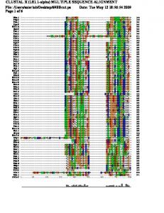
Figure 9 –Visual comparison of the alignment produced by the GA (a) and the alignment produced by ClustalW (b). Although extremely similar, the GA alignment is slightly more optimal. For example, the alignment produced by Clustal W has one additional column, indicating that more gaps were used to construct the alignment. The slight improvement in alignment quality is also apparent on a closer visual inspection.
10
7
Conclusions
We have presented a novel and highly effective approach to applying genetic algorithms to the problem of progressive multiple sequence alignment. In addition, we have presented a novel use of a binary coalescent tree as a data structure which lends itself nicely to the problem of performing crossover on two trees without duplicating terminal nodes. In our tests, our evolutionary approach has been shown to produce more refined alignments than ClustalW. In addition, we believe that preliminary execution time data seem to indicate a trend that our approach may be more scalable than ClustalW when aligning very large numbers of very long sequences, although more work must be performed to make a conclusive determination on the relative scalability of our technique.
8
Future Work
Our approach produced higher-scoring alignments than ClustalW while also being more scalable than ClustalW for extremely large datasets (i.e. 500 sequences or more). Additional testing needs to be done in order to determine the precise inflection point at which our approach surpasses ClustalW in both alignment quality and scalability for different input sizes. We intend to study the parameterization of our GA in greater detail to determine how best to converge to a near-optimal guide tree in the minimum number of iterations. The effects of modifying tunable parameters such a population size and mutation rate on solution convergence rates and solution quality will be more fully explored. Additionally, we intend to explore new styles of crossover and mutation operators based on coalescing trees in order to maximize the benefits of those operators. Although our internal coalescing tree representation is novel and has certain advantages, the ability of our representation to take full advantage of the theoretical principles of evolutionary computation (i.e. the building block hypothesis) is uncertain. Preliminary empirical evidence indicates that our crossover operator in combination with our tree representation may have weak building block properties, leading us to us believe that the crossover operator and internal tree representation presented herein is relatively inefficient and may cause the GA to perform only slightly better than a parallel hill climb. In future work, we intend to implement the tree crossover operator described by Lewis in his GAML system [9]. Lewis successfully reconstructed phylogenetic trees with genetic algorithms using a modified form of inter-tree tree bisection and recombination (TBR) for crossover. We intend to compare and contrast the efficiency of Lewis’s crossover approach with our own. Currently, this GA is designed to handle only nucleotide sequences. We intend to extend this algorithm to handle protein sequence data as well, with support for fully pluggable amino acid substitution matrices (such as BLOSSUM and PAM). Once this GA supports the alignment of amino acid sequences, we intend to perform benchmarked comparisons against other techniques using the BAliBASE [8] alignment database. The problem of sequence alignment is embarrassingly parallel. Genetic algorithms are also inherently parallel, and so we intend to parallelize our fitness function such that it can be efficiently handled in a Beowulf cluster configuration. 11
Finally, we will examine the effects of evolving guide trees whose fitness is evaluated by some measure of fitness distinct from final alignment quality. Other fitness criteria for applying evolutionary pressure to improving guide trees may be equally effective in achieving high-quality alignments, and perhaps considerably faster.
Acknowledgments Special thanks to Jason Evans and Conrad Shyu from the University of Idaho for fruitful brainstorming sessions and implementation review. This research used equipment funded in part by NIH NCRR 1P20 RR16448, and NIH NCRR 1P20 RR16454. Sheneman was partially funded by NIH NCRR 1P20 RR16448. Foster was partially funded for this research by NIH NCRR 1P20 RR16448.
9
Bibliography
[1] Thomson, J.D., Higgins D.H., and Gibson, T.J., “CLUSTAL W: Improving the sensitivity of progressive multiple sequence alignment through sequence weighting, position-specific gap penalties and weight matrix choice”, Nucleic Acids Research, 1994, Vol 22, No 22 4673-4680 [2] Needleman, S.B. and Wunsch, C.D., “A general method application to the search for similarities in the amino acid sequences of two proteins”, Journal of Molecular Biology, 1970, 48(3):443-53 [3] Smith, T.F., Waterman, M.S., “Identification of Common Molecular Subsequences”, Journal of Molecular Biology, 1981, 48:443-453 [4] Saitou, N., and Nei, M., “The neighbor-joining method: a new method for reconstructing phylogenetic trees”, Journal of Molecular Biology Evolution, 1987, 4:406-425 [5] Thomsen, R., Fogel, G.B., Krink, T., “A Clustal Alignment Improver using Evolutionary Algorithms”, In Proceedings of the Fourth Congress on Evolutionary Computation (CEC-2002), 2002, vol. 1, pp 121-126 [6] Kececioglu, J.D., and Zhang, W., “Aligning Alignments”, Proceedings of the 9th Annual Symposium on Combinatorial Pattern Matching (CPM ’98), 1998 [7] Jukes, T.H., and Cantor, C., “Evolution of protein molecules”, In H.N. Munro (Ed), Mammalian Protein Metabolism, Volume III, Chapter 24, pp. 21-132, Academic Press, New York [8] Thomson, J.D., Plewniak, F., and Poch O., “BAliBASE: a benchmark alignment database for the evaluation of multiple alignment programs”, Bioinformatics, 15(1): 87-88, 1999 [9] Lewis, P.O., “A Genetic Algorithm for Maximum-Likelihood Phylogeny Inference Using Nucleotide Sequence Data”, Molecular Biology Evolution, 15(3):277-283, 1998 [10] Holland, J.H., Adaptation in Natural and Artificial Systems, University of Michigan Press, 1975
12