Exploiting Heterogeneity for Adaptive Calibration

Exploiting Heterogeneity for Adaptive Calibration in Wireless Sensor Networks Rui Tan1 Guoliang Xing2 Xue Liu3 Jianguo Yao4 Zhaohui Yuan5 1 City University of Hong Kong, HKSAR 2 Michigan State University, USA 3 McGill University, Canada 4 Northwestern Polytechnical University, P.R. China 5 Wuhan University, P.R. China I. I NTRODUCTION Wireless sensor networks (WSNs) are increasingly deployed in mission-critical applications such as target detection, tracking and security surveillance. In these applications, the sensing performance of a network is inherently affected by stochastic sensor noises, unpredictable environment changes and dynamics of the monitored phenomenon. In order to achieve desirable system performance, the operational parameters of a network must be dynamically calibrated in response to these uncertainties. Advanced collaborative signal processing algorithms such as data fusion [1] have been proposed to mitigate the impact of noise by jointly considering the measurements of multiple sensors. However, these algorithms are not designed to handle hardware biases or environmental dynamics. Sensor calibration [2] can correct hardware biases by tuning each individual sensor based on ground truth information about physical processes. However, the ground truth information is often unknown or subject to dynamic evolution in reality, which often leads to unpredictable system performance at run time. In this paper, we exploit sensor heterogeneity to achieve adaptive calibration performance for surveillance WSNs. Many practical WSNs have multiple sensor modalities. For instance, a typical surveillance system [3] has both low-end passive infrared sensors and high-quality pan-tilt-zoom cameras. Lowend sensors consume less energy but often have limited sensing capability such as high false alarm rate. In contrast, high-quality sensors can yield high-fidelity measurements at the price of high energy consumption. In our calibration approach, lowend sensors collaboratively detect targets through data fusion [1]. When a positive detection consensus is reached by lowend sensors, high-quality sensors are activated to make a highfidelity detection. The low-end sensors are then iteratively calibrated according to the detection results of high-quality sensors. In particular, the high-quality sensors are allowed to sleep for most of the time and only activated when a possible target is detected by low-end sensors. Such a two-tier calibration framework can significantly reduce system energy consumption while maintaining satisfactory surveillance performance. We formally formulate the problem of adaptive calibration as a control problem. The system objective is to maximize the detection performance and adapt to dynamic network conditions and physical environments. We develop a control-theoretical solution with provable system stability and convergence. We also systematically analyze the impacts of communication reliability and delay. Moreover, we propose an optimal routing algorithm that minimizes the impact of packet loss on system stability. We conduct experiments on a testbed of Tmotes as

well as trace-driven simulations using real data traces collected in a vehicle detection experiment [4]. The results show that the calibrated network maintains optimal detection performance in the presence of various system and environmental dynamics such as link reliability, delay, and target mobility. II. P ROBLEM F ORMULATION

AND

A PPROACH OVERVIEW

We assume that the heterogeneous WSN is composed of N low-end sensors and a high-quality sensor. The objective is to detect targets that randomly appear. The probability that the target appears at any time instance is Pa . Depending on the hypothesis that the target is absent (H0 ) or present (H1 ), the measurement of low-end sensor i, denoted by yi , is given by 

H0 : H1 :

yi = ni , yi = si + ni ,

where si and ni are the energies of signal and noise received by sensor i, respectively. We assume that ni follows the normal distribution, i.e., ni ∼ N (µi , σi2 ), where µi and σi2 are the mean and variance of ni , respectively. The low-end sensors collaboratively detect targets by fusing their measurements. Let P Y denote the sum of their measurements (i.e., Y = N i=1 yi ) and T denote the detection threshold at the cluster head. If Y ≥ T , the cluster head decides H1 ; otherwise, it decides H0 . Our objective is to find the optimal detection threshold at the cluster head such that the average error rate PE , i.e., the probability that the cluster head makes wrong detection decision, is minimized. From the Bayesian detection theory [1], the optimal detection threshold Topt that minimizes PE is given P PN 2 2 2 + µ + S2 , where µ =” N by Topt = δσ i=1 µi , σ = i=1 σi , 2S “ PN 1−Pa S = . However, the optimal i=1 si and δ = 2 ln Pa detection threshold Topt is often unknown and cannot be easily estimated in practice. This is because, first, the noise profiles, i.e., µ and σ 2 , are often unknown and can change at run time. Second, the aggregated signal energies, i.e., S , depends on the source energy and position of the target which are also unknown variables. As a result, implementing the optimal detector based on unknown µ, σ 2 and S is largely unpractical in practice. In this paper, we exploit sensor heterogeneity to overcome the difficulties caused by the unknown variables µ, σ 2 and S. As the high-quality sensor can detect the target accurately, the detection results can be fed back to calibrate the low-end sensors when the target profiles and environment conditions have changed. Our problem is formally formulated as follows. Problem 1. To find the stable and converging calibration algorithm for the detection threshold T at the cluster head based on the feedback of the high-quality sensor, such that the average error rate PE is minimized.

2

We propose a calibration approach that features feedback control loop to solve Problem 1, where the controller is implemented by the calibration algorithm located at the cluster head. The overview of our approach is as follows. The detection threshold T is calibrated iteratively for every calibration cycle. Each calibration cycle comprises a number of detections. In each detection, the cluster head fuses the measurements received from the low-end sensors to make a detection decision by comparing against the current detection threshold T . Only if the cluster head makes a positive detection decision, the highquality sensor is activated to make a detection and reports its decision to the cluster head. At the end of each calibration cycle, the cluster head estimates the detection performance of low-end sensors, which is characterized by the false alarm rate and missing probability, according to the detection history and the feedback of the high-quality sensor. The cluster head then calibrates the detection threshold T according to the difference between the estimated and the optimal detection performances. III. A DAPTIVE C ALIBRATION A LGORITHM A. Modeling Feedback of High-quality Sensor In this section, we derive the estimates of false alarm rate and missing probability of the low-end sensors, denoted by PF L and PM L , respectively, which are used as the feedback of the highquality sensor. At the end of a calibration cycle, the cluster head counts the numbers of positive and negative decisions made by the high-quality sensor and estimates PF L and PM L based on the counts. We assume that the false alarm rate and missing probability of the high-quality sensor, denoted by PF H and PM H , are known. For instance, they can be measured via offline experiments. We define the following notation subject to a calibration cycle: 1) nf 1 and nd1 are the numbers of false alarms and correct detections made by the cluster head, respectively, which are unknown; 2) nf 2 and nd2 are the numbers of positive decisions made by the cluster head but regarded to be false alarms and correct detections by the highquality sensor, respectively, which can be counted by the cluster head. We have the following equations, nf 2 ≃ nf 1 (1 − PF H ) + nd1 PM H , nd2 ≃ nf 1 PF H + nd1 (1 − PM H ).

(1) (2)

From (1) and (2), nf 1 and nd1 can be estimated as nf 1 ≃

nd2 (1−PF H )−nf 2 PF H nf 2 (1−PM H )−nd2 PM H , nd1 ≃ . 1−PF H −PM H 1−PF H −PM H

Therefore, PF L and PM L can be estimated as PF L ≃

nf 1 , m − m · Pa

PM L ≃

m · Pa − nd1 , m · Pa

(3)

where m is the number of detections in a calibration cycle. B. Control Law and Adaptive Calibration Algorithm We first investigate the relationship between PF L and PM L when the average error rate is minimized. We have the following lemma. The proof is omitted and can be found in [5]. Lemma 1. The average error `rate PE is´ minimized if and ` ´2 2 only if V“ = δ,” where V = Q−1 (PF L ) − Q−1 (PM L ) , a and Q−1 (·) is the inverse function of the δ = 2 ln 1−P Pa complementary CDF of the standard normal distribution. From Lemma 1, the performance objective of Problem 1 can be reduced to V = δ , where the performance metric V

δ

+ h− 6

T Gc (z)

-

Gp (z)

q

V

-

H(z)

Fig. 1.

The closed-loop system for minimizing PE .

depends on the detection threshold T and can be estimated based on the feedback of the high-quality sensor as discussed in Section III-A. Moreover, the detection threshold T is calibrated for every calibration cycle. Therefore, Problem 1 is a typical discrete-time control problem [6], in which δ is the reference, T is the control input and V is the controlled variable. The block diagram of the feedback control loop is shown in Fig. 1, where Gc (z), Gp (z) and H(z) represent the transfer functions of the calibration algorithm (i.e., controller), the network of low-end sensors and the feedback of high-quality sensor, respectively. The transfer function Gp (z) can be derived by analyzing the detection performance of the low-end sensors given detection threshold T . Specifically, it is given by Gp (z) = σ2S2 (the derivation can be found in [5]). At the end of a calibration cycle, the cluster head computes V based on the estimated PF L and PM L as discussed in Section III-A. Accordingly, the feedback of the high-quality sensor will take effect in the next calibration cycle. Therefore, the H(z) has a component of z −1 that represents a delay of one calibration cycle. We ignore the inaccuracy in estimating V and hence H(z) = z −1 . As the system to be controlled, i.e., Gp (z), is a zero-order system, a first-order controller is sufficient to achieve system stability a and convergence [6]. Hence, we let Gc (z) be Gc (z) = 1−b·z −1 , where a and b are two parameters to be determined. The system 2 is stable and converging if 0 < a < σS and b = 1. The stability and convergence analyses are omitted here and can be found in [5]. To achieve short system response delay, the best setting for 2 a is a value close to the upper bound σS . However, the upper bound is unknown. From the expression of Gp (z), the ratio σ2S2 can be estimated from the inputs and outputs of Gp (z), and then 2 can be used to estimate the upper bound σS . Due to space limit, the details are omitted here and can be found in [5]. Finally, we implement the control law as the adaptive calT (z) a ibration algorithm. As Gc (z) = δ−H(z)V = 1−b·z −1 and (z) ` ´ −1 −1 H(z) = z , we have T (z) = b · z T (z) + a · δ − z −1 V (z) and its implementation in time domain is T [k] = b · T [k − 1] + a · ` ´2 ` ´2 (δ − V [k − 1]), where V [k − 1] = Q−1 (PF L ) − Q−1 (PM L ) , th T [k−1] and T [k] are the detection thresholds in the (k−1) and k th calibration cycle, respectively. PF L and PM L are computed using (3) when the detection threshold is T [k − 1]. Note that 2 b = 1 and a is set to be a value close to σS , as discussed above. C. Impact of Communication Performance In this section, we study the impacts of packet loss and feedback delay on our calibration algorithm. The details of the analysis can be found in [5] and we only summarize the results here. First, from Section III-B, the system stability is 2 affected by the upper bound of a, i.e., σS . In the presence of stochastic packet loss, both S and σ 2 can change rapidly and hence the system may become unstable. The relative standard deviations (RSDs) of S and σ 2 , which characterize their change

3

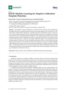
200 150 100

sensors cluster head AAV

50

0 50 100 150 200 250 300 350 400 West-East (meters)

Fig. 2.

Sensor deployment [4].

T 2

0.8 0.7 0.6 0.5 0.4 0.3 0.2 0.1

1

offline optimal our approach heuristic 0

50 100 200 300 400 500 m

RMSD(PE ) vs. m.

Fig. 3.

“

”

magnitudes, are RSD(S) = RSD(σ 2 ) = O √1N . Therefore, the impact of packet loss can be mitigated by deploying more low-end sensors. Second, the optimal routing path for sensor i, that minimizes RSD(S) and RSD(σ 2 ), is the shortest path to the cluster head where the cost of hop h is − log PRR(h) and PRR(h) is the packet reception rate of hop h. Third, the communication delay can be modeled as the delay of feedback, and its impact on the system stability can be analyzed via the Jury test [6]. The system stability decreases with the delay. IV. P ERFORMANCE E VALUATION We have implemented the calibration algorithm on a small testbed of Tmote Sky motes. The details of the testbed experiments can be found in [5]. In this section, we only present the extensive simulations based on real data traces. A. Simulation Methodology and Settings We use the real data traces collected in the DARPA SensIT vehicle detection experiment [4], where 75 WINS NG 2.0 nodes are deployed to detect Amphibious Assault Vehicles (AAVs) driving through a road section. The dataset used in our simulations includes the ground truth data and the acoustic time series recorded by 17 nodes. The ground truth data include the positions of sensors and the trajectory of the AAV recorded by a GPS device. Fig. 2 [4] shows the sensor deployment and the trajectory of an AAV run. The AAV is regarded to be present when it is in the circular region in Fig. 2. The target appearance probability Pa is set to be 25%. As there is no extra highquality sensor such as camera in the SensIT experiment, we use a pseudo camera in the simulations, which generates random detection results based on the ground truth data. The pseudo camera’s false alarm rate and missing probability, i.e., PF H and PM H , are both set to be 1%. We employ a heuristic calibration approach as the baseline, in which the noise profiles (i.e., µ and σ 2 ) and aggregated signal energies (i.e., S ) are directly estimated from the noisy measurements, according to the detection results of the highquality sensor [5]. The detection threshold is then set according to the optimal formula given in Section II with the estimates. B. Simulation Results The first set of simulations evaluate the performance of our calibration approach in detecting moving targets. Fig. 4 plots the evolution of detection thresholds calibrated by various approaches. The offline optimal approach computes the optimal detection threshold based on the S, µ and σ 2 that are estimated from ground truth data. From the figures, we can see that our

20

optimal routing baseline

40

20

0

30

40

50

Detection threshold T vs. index of calibration cycle. 3

60 0

10

Fig. 4. RMSD of PE (%)

250

0

our approach heuristic

3

300

RMSD of PE (%)

South-North (meters)

350

RMSD of PE (%)

400

2

1

0 6 7 8 9 10 11 12 13 14 PT x (dBm)

Fig. 5.

RMSD(PE ) vs. PT x .

0

2

Fig. 6.

4 6 Delay d

8

10

RMSD(PE ) vs. d.

approach converges to the optimal results after 10 calibration cycles and can adapt to the dynamics of target. In constrast, the heuristic approach has considerably large steady-state error. The second set of simulations evaluate the impact of several affecting issues. We employ the root mean square deviation (RMSD) of PE with respect to the offline optimal approach as the performance metric. We first evaluate the impact of m, i.e., the number of detections in a calibration cycle. Fig. 3 plots the RMSD(PE ) versus m. The system shows better convergence for larger m. Moreover, our approach yields smaller RMSD(PE ) than the heuristic approach under a wide range of m. We then evaluate the impact of packet loss. We employ the link model in [7] to compute the PRR of each link in the network. The routing path from each sensor to the cluster head (shown in Fig. 2) is computed by Dijkstra’s algorithm. Besides the optimal routing algorithm, we employ a baseline 1 . Fig. 5 routing algorithm in which the cost of link h is PRR(h) plots the RMSD(PE ) under various routing algorithms versus the transmission power PT x at each sensor. We can see from the figure that our approach with the optimal routing algorithm converges when the PT x is no lower than 9 dBm. However, the system shows considerably large deviation when the baseline routing algorithm is used. We finally evaluate the impact of feedback delay. Specifically, the feedback information is delayed for d calibration cycles. Fig. 6 plots the RMSD(PE ) versus the delay d. We can see that our calibration algorithm is robust to feedback delay. Specifically, the RMSD(PE ) increases 1% even if the delay is 10 calibration cycles. R EFERENCES [1] P. K. Varshney, Distributed Detection and Data Fusion. Springer, 1996. [2] K. Whitehouse and D. Culler, “Calibration as parameter estimation in sensor networks,” in WSNA, 2002. [3] C. Wren, U. Erdem, and A. Azarbayejani, “Functional calibration for pantilt-zoom cameras in hybrid sensor networks,” Multimedia Systems, vol. 12, no. 3, 2006. [4] M. Duarte and Y.-H. Hu, “Vehicle classification in distributed sensor networks,” J. Parallel and Distributed Computing, vol. 64(7), 2004. [5] R. Tan, G. Xing, X. Liu, J. Yao, and Z. Yuan, “Adaptive calibration for fusion-based wireless sensor networks,” City University of Hong Kong, Tech. Rep., 2009, http://www.cs.cityu.edu.hk/∼ tanrui/pub/camdetect.pdf. [6] K. Ogata, Discrete-time control systems. Prentice-Hall, 1995. [7] M. Zuniga and B. Krishnamachari, “Analyzing the transitional region in low power wireless links,” in SECON, 2004.