Performance of the Parallel Bootstrap Simulation Algorithm. The 12th IEEE ... Hybrid programming model with MPI and Open
Exploiting Multi-core Architectures in Clusters for Enhancing the Performance of the Parallel Bootstrap Simulation Algorithm The 12th IEEE International Workshop on Parallel and Distributed Scientific and Engineering Computing (PDSEC 2011)
C´esar A. F. De Rose, Paulo Fernandes, Antonio M. Lima, Afonso Sales, Thais Webber (Avelino F. Zorzo)
Pontif´ıcia Universidade Cat´olica do Rio Grande do Sul (PUCRS) PaleoProspec Project - PUCRS/Petrobras Funded also by CAPES and CNPq - Brazil
Context Interest The solution of complex and large state-based stochastic models to extract performance indices.
Application domains Biology, Physics, Social Sciences, Business, Computer Science and Telecommunication, etc.
Modeling Examples ASP - Alternate Service Patterns: describes an Open Queueing Network with servers that map P different service patterns FAS - First Available Server: indicates the availability of N servers RS - Resource Sharing: maps R shared resources to P processes
Context Problem large amount of possible configurations of large models a traditional numerical solution becomes intractable and easily dependable on the available computational resources
Solution alternatives Numerical: bounded by memory
Simulation: lack of accuracy
and computational power
generating samples
Iterative methods:
Methods:
◮ ◮ ◮
Power [Stewart 94] GMRES [Saad and Schultz Arnoldi [Arnoldi 51]
◮
86]
◮ ◮ ◮
Traditional [Ross 96] Monte Carlo [H¨aggstr¨om 02] Backward [Propp and Wilson 96] Bootstrap [Czekster et al. 10] ⋆ ⋆
reliable estimations high computational cost to generate repeated batches of samples
Context
Simulation of Markovian models Definitions: initial state, trajectory length (number of samples) Main idea: perform a random walking process given the set of possible states that the system assumes (simulation trajectory) computing an approximation of the steady-state probability distribution Generation of independent samples for later statistical analysis Large models imply large memory costs Remark: need long run trajectories for more accuracy results
Outline Goal Faster numerical solution using the Bootstrap simulation algorithm, exploiting parallelism in a multi-core SMP cluster
Strategy Parallel approaches: using only MPI primitives Hybrid programming model with MPI and OpenMP: ◮ ◮
fine grain (Hybrid-I) coarse grain (Hybrid-II)
Results and Discussion Performance issues of the parallel Bootstrap implementations
Bootstrap simulation Algorithm Schema States
Bootstrapping process
Initial state
s2
K1
s2
s1
s1
s1
s0
s0
s0
1
2
s1
...
s0
s1
. . . s1
s2
s2
Time 0
3 ...
n
π x¯1[0] + x¯2[0] + ··· + x¯z [0] z π1 x¯1[1] + x¯2[1]z+ ··· + x¯z [1] π2 x¯1[2] + x¯2[2] + ··· + x¯z [2] z
π0
Kz
s0
Normalization
s2
x¯1 Computing
x¯z
s0
s0
s1
. . . s1
s2
s2
01. 02. 03. 04. 05. 06. 07. 08. 09. 10. 11. 12. 13. 14. 15. 16. 17. 18. 19. 20. 21. 22. 23. 24. 25. 26.
α ← U (0..¯ n-1) π←0 K←0 s ← s0 for t ← 1 to n do snew ← φ(s, U (0..1)) for b ← 1 to z do for c ← 1 to n ¯ do if (U (0..¯ n − 1) == α) then Kb [snew ] ← Kb [snew ] + 1 end for end for s ← snew end for for b ← 1 to z do ω←0 for i ← 1 to |S| do ω ← ω + Kb [i] for i ← 1 to |S| do x ¯b [i] ← Kωb [i] end for for i ← 1 to |S| do for b ← 1 to z do π[i] ← π[i] + x ¯b [i] π[i] ← π[i] z end for
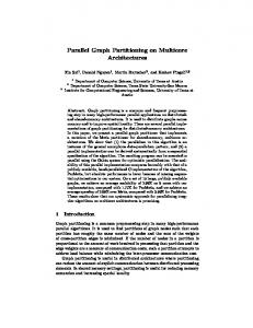
Bootstrap simulation Processing costs Times vs. Max. Absolute Error 100000
4.50e-03 4.00e-03
the number of trials (¯ n) in the resampling process
1000 2.50e-03 2.00e-03 100 1.50e-03 1.00e-03
10
5.00e-04 1
0.00e+00 1e+09
1e+08
1e+07
FAS model
1e+06
1e+05
1e+09
1e+08
1e+07
1e+06
1e+05
ASP model
1e+09
1e+08
1e+07
1e+06
1e+05
z×n ¯ samplings take place for every trajectory step
3.50e-03 3.00e-03
Time (s)
the number of bootstraps (z)
10000
Maximum Absolute Error
the trajectory length (n)
RS model
Simulation trajectory length
Proposal Parallel Bootstrap implementations that change the workload distribution and programming model
Parallel approaches Environment Multi-core SMP cluster 8 nodes (Gigabit Ethernet network) Each node has two Intel Xeon E5520 Quad-core - Hyper-Threading technology - 16 logical processors - 16 GB RAM Linux O.S. OpenMPI 1.4.2
Number of bootstraps assigned to nodes in each configuration configuration 1 2 3 4 5 6 7 8
number of bootstraps 36 18 12 9 7 6 5 4
18 12 9 7 6 5 4
12 9 7 6 5 4
9 7 6 5 4
8 6 5 5
OpenMP 2.5
Experiments 30 trials taking a 95% confidence interval 1 (sequential), 2, 3, 4, 5, 6, 7, and 8 nodes z = 36 bootstraps and n=1e+06, 1e+07, 1e+08, and 1e+09
6 5 5
6 5
5
Parallel approaches (pure-MPI)
Pure MPI implementation Node #1 Bootstrapping process (sequential computation)
Split the bootstrap sampling tasks over C processing nodes Node #2
# bootstraps
Bootstrapping process (sequential computation) ... ... .. . ...
... ... .. . ...
Node #C Bootstrapping process (sequential computation) # bootstraps
# bootstraps
Only MPI primitives
... ... .. . ...
Parallel approaches (pure-MPI results) Large models (millions of states)
Small models (hundreds of states)
n = 1e+06
n = 1e+06
30
30
Next-State Bootstrapping Normalization Communication Computing
25
20
Time (s)
Time (s)
20
15
15
10
10
5
5
0
0 1
2
3
4 5 ASP
6
7
8
1
2
3
4 5 FAS
6
7
8
1
2
3
4 5 RS
6
7
8
1
2
3
4 5 ASP
6
7
8
1
2
3
4 5 FAS
6
7
8
Configuration
Configuration
n = 1e+09
n = 1e+09
18000
1
18000
Next-State Bootstrapping Normalization Communication Computing
16000 14000
14000
12000
12000
10000 8000
3
4 5 RS
6
7
8
7
8
10000 8000
6000
6000
4000
4000
2000
2
Next-State Bootstrapping Normalization Communication Computing
16000
Time (s)
Time (s)
Next-State Bootstrapping Normalization Communication Computing
25
2000
0
0 1
2
3
4 5 ASP
6
7
8
1
2
3
4 5 FAS
6
7
Configuration
8
1
2
3
4 5 RS
6
7
8
1
2
3
4 5 ASP
6
7
8
1
2
3
4 5 FAS
6
7
Configuration
8
1
2
3
4 5 RS
6
Parallel approaches (fine grain) Hybrid MPI/OpenMP implementation (Hybrid-I) Hybrid programming
Node #1 Bootstrapping process (parallel computation)
MPI and OpenMP
...
...
...
...
... .. . ...
... .. . ...
... .. . ...
... .. . ...
loop at line 7
... for t ← 1 to n do snew ← φ(s, U (0..1)) for b ← 1 to z do for c ← 1 to n ¯ do if (U (0..¯ n − 1) == α) then Kb [snew ] ← Kb [snew ] + 1 end for end for s ← snew end for ...
Node #2
Node #C
Bootstrapping process (parallel computation) # threads
◮ 04. 05. 06. 07. 08. 09. 10. 11. 12. 13. 14. 15.
# threads
Intra-node parallelism #pragma omp parallel for
...
...
...
...
... .. . ...
... .. . ...
... .. . ...
... .. . ...
Bootstrapping process (parallel computation) # threads
◮
...
...
...
...
... .. . ...
... .. . ...
... .. . ...
... .. . ...
Parallel approaches (Hybrid-I results)
n = 1e+06
n = 1e+09
70
70000
Next-State Bootstrapping Normalization Communication Computing
60
50000
Time (s)
50
Time (s)
Next-State Bootstrapping Normalization Communication Computing
60000
40
30
40000
30000
20
20000
10
10000
0
0 1
2
4 ASP
8
1
2
4
8
1
FAS
Number of threads in only one node
2
4 RS
8
1
2
4 ASP
8
1
2
4
8
1
FAS
2
4
8
RS
Number of threads in only one node
A parallel region is created at each step in the simulation process
Parallel approaches (coarse grain) Hybrid MPI/OpenMP implementation (Hybrid-II) Hybrid programming MPI and OpenMP
Node #1 Bootstrapping process (parallel computation) ...
...
...
...
... .. . ...
... .. . ...
... .. . ...
... .. . ...
lines 5 to 14
... for t ← 1 to n do snew ← φ(s, U (0..1)) for b ← 1 to z do for c ← 1 to n ¯ do if (U (0..¯ n − 1) == α) then Kb [snew ] ← Kb [snew ] + 1 end for end for s ← snew end for ...
Node #2
Node #C
Bootstrapping process (parallel computation) # threads
◮ 04. 05. 06. 07. 08. 09. 10. 11. 12. 13. 14. 15.
# threads
Intra-node parallelism Parallel region integrates the whole simulation process
...
...
...
...
... .. . ...
... .. . ...
... .. . ...
... .. . ...
Bootstrapping process (parallel computation) # threads
◮
...
...
...
...
... .. . ...
... .. . ...
... .. . ...
... .. . ...
Parallel approaches (Hybrid-II results) Large models
Small models
n = 1e+06
n = 1e+06 Next-State + Bootstrapping Normalization Communication Computing
10
10
8
8
6
6
4
4
2
2
8 (5)
7 (6)
8 (5)
2500
Next-State + Bootstrapping Normalization Communication Computing
2000
1500
1500
Time (s)
Time (s)
7 (6)
6 (6)
5 (8)
4 (9)
3 (12)
2 (16)
1 (16)
8 (5)
7 (6)
6 (6)
5 (8)
4 (9)
RS
n = 1e+09
2000
1000
500
Next-State + Bootstrapping Normalization Communication Computing
1000
500
RS
6 (6)
5 (8)
4 (9)
3 (12)
2 (16)
FAS
Configuration (Threads)
1 (16)
8 (5)
7 (6)
6 (6)
5 (8)
4 (9)
3 (12)
2 (16)
1 (16)
8 (5)
7 (6)
ASP
6 (6)
5 (8)
4 (9)
3 (12)
2 (16)
0
1 (16)
8 (5)
7 (6)
RS
6 (6)
5 (8)
4 (9)
3 (12)
2 (16)
FAS
Configuration (Threads)
1 (16)
8 (5)
7 (6)
6 (6)
5 (8)
4 (9)
3 (12)
2 (16)
1 (16)
8 (5)
7 (6)
ASP
6 (6)
5 (8)
4 (9)
3 (12)
2 (16)
1 (16)
0
FAS
Configuration (Threads)
n = 1e+09 2500
3 (12)
2 (16)
ASP
Configuration (Threads)
1 (16)
8 (5)
7 (6)
6 (6)
5 (8)
4 (9)
3 (12)
RS
2 (16)
1 (16)
0
8 (5)
7 (6)
6 (6)
5 (8)
4 (9)
3 (12)
2 (16)
FAS
1 (16)
8 (5)
7 (6)
6 (6)
5 (8)
4 (9)
3 (12)
2 (16)
ASP
1 (16)
8 (5)
7 (6)
6 (6)
5 (8)
4 (9)
3 (12)
2 (16)
1 (16)
0
Next-State + Bootstrapping Normalization Communication Computing
12
Time (s)
Time (s)
12
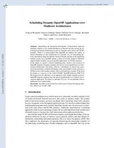
Parallel approaches (Hybrid-II results)
Speedup vs. Efficiency Large models (n = 1e+09) 40
Small models (n = 1e+09) 120
35
100
30
100 90
35
80 30
70
40
Speedup
Speedup
20
25 60 20
50 40
15 30
15
20 10
20
10
0
5
10 5 1 2 3 4 5 6 7 8 ASP
1 2 3 4 5 6 7 8 FAS
Configuration
1 2 3 4 5 6 7 8 RS
0 1 2 3 4 5 6 7 8 ASP
1 2 3 4 5 6 7 8 FAS
Configuration
1 2 3 4 5 6 7 8 RS
Efficiency (%)
60
Efficiency (%)
80 25
Conclusion and future works
Summary Parallel performance analysis of the Bootstrap simulation algorithm, exploiting different characteristics of multi-core SMP clusters The algorithm allows the generation of samples in an independent manner, which is trivial in terms of parallelization efforts Considerable speedups have been achieved for very large models Processing demands depend only on the trajectory length (n) Communication demands depend only on the size of the model
Conclusion and future works
Future works Practical ◮ ◮
an efficient implementation of transition function to compute samples adapting parallel sampling techniques to mitigate the efforts related to the simulation of structured Markovian models
Theoretical ◮
◮
further study may be considered about the impact of the number of bootstraps on the accuracy of the simulation results incorporate the parallel sampling process with more sophisticated simulation approaches, such as Perfect Sampling
Thank you for your attention