Oct 11, 2013 - sition (SCADA) system data for performance monitoring of large utility-scale wind turbines. The general approach taken is to model the turbine ...
2013 Conference on Control and Fault-Tolerant Systems (SysTol) October 9-11, 2013. Nice, France
Exploiting SCADA System Data for Wind Turbine Performance Monitoring Shane Butler1 , John Ringwood1 and Frank O’Connor2 each individual turbine. The specific behaviour modelled is the relationship between input variables, comprising weather measurements and turbine sensor measurements, and the mean power generated by each turbine. By modelling the fault-free behaviour of each individual wind turbine, each trained model can then be used to monitor the performance of each respective turbine going forward. By monitoring the characteristics of the residual signal, which represents the difference between the predicted and observed power produced by the turbine at each time-step, it may be possible to identify subsequent turbine performance degradation which impacts upon the power generated by the turbine. Wind turbine power curve analysis is a common method for providing a universal measure of wind turbine performance and as an indicator of overall wind turbine health [8]. The wind power curve, for a specific wind turbine device, relates the turbine power output for a given wind speed. Given the current wind conditions, differences between the expected power output, as estimated by the power curve, and the actual power output are identified and have previously been used to indicate potential operational issues, such as the overall blade condition [2] and gearbox faults [8]. The use of turbine SCADA information has also become more widespread with authors exploiting such data for gearbox, generator, and bearing component fault detection and prediction applications [10], [4], [1]. The layout of the remaining sections of this paper are as follows: Section II presents some details on the proposed wind turbine performance monitoring algorithm. Section III describes the data filtering process necessary to identify suitable data samples for analysis. Section IV describes the use of Gaussian process models to model turbine power output. Section IV-B describes the process of identifying suitable model inputs for modelling turbine power output. Finally, Section V presents some results of the algorithm tested on historical turbine failure examples.
Abstract— This paper presents the results of a short study into utilising wind farm supervisory control and data acquisition (SCADA) system data for performance monitoring of large utility-scale wind turbines. The general approach taken is to model the turbine power output of each turbine during fault-free operation and to subsequently use the trained model to identify performance degradation by analysing the residual between the predicted and observed power values for each turbine. Historical data from a large wind farm is used to train and test the turbine models. The trained models are then tested on historical turbine failure examples. The results suggest that the data collected by wind farm SCADA systems, which are typically installed as standard on most modern wind farms, can be exploited for gaining an insight into wind turbine performance and maintenance condition.
I. INTRODUCTION Over the past decade, the deployed wind power generating capacity worldwide has increased rapidly. By the end of 2010, wind generating capacity reached approximately 196,630 MW [9]. In addition, the size and generating capacity of individual wind turbines also continues to increase, with increasing numbers of wind turbines with >5MW generating capacity becoming standard in offshore wind farms. For offshore wind farms, studies have suggested that maintenance costs are about 20 to 25% of the total income generated, and that a considerable percentage of these costs are due to unexpected equipment failure, which require corrective maintenance [6]. In an effort to reduce the maintenance costs for wind turbines, wind farm operators are increasingly embracing condition-based maintenance philosophies in an effort to reduce maintenance costs, increase turbine reliability, and reduce turbine downtime and associated loss of revenue. Most modern turbines incorporate onboard supervisory control and data acquisition (SCADA) systems for control and monitoring. As these system are already installed as standard, wind farm operators are increasingly interested in better exploiting this data for condition monitoring, fault diagnostics, and fault prognostics. In this paper, the development of a wind turbine performance monitoring algorithm using SCADA system measurements from a large wind farm is described. The general principle of the approach is to model the fault-free behaviour of
II. A WIND TURBINE PERFORMANCE MONITORING ALGORITHM In this study, historic SCADA system data from a large wind farm was made available. For each turbine in the wind farm, the complete history of sensor information and turbine status information, for a period of 24-months, was available. The onboard SCADA system for each turbine records 10minute averages of each monitored sensor variable. Figure 1 presents a flow chart describing the proposed wind turbine performance monitoring algorithm. At 10minute intervals, the latest SCADA measurements are gen-
*This work was supported by Enterprise Ireland 1 Shane Butler and John Ringwood are with the Department of Electronic Engineering, National University of Ireland, Maynooth, Maynooth, Co. Kildare, Ireland shane.butler at eeng.nuim.ie 2 Frank O’Connor is with ServusNet Informatics Ltd, National Software Centre, Mahon, Co. Cork, Ireland frankoconnor at
servusnet.com 978-1-4799-2854-5/13/$31.00 ©2013 IEEE
389
Data Filtering
Proposed wind turbine performance monitoring algorithm
erated at each turbine. The first step is a filtering step to select only those samples which satisfy a number of status requirements. Section III describes this filtering step in more detail. If the turbine operating status requirements for the latest SCADA measurement are satisfied, then the latest SCADA data sensor measurements are passed as inputs to the Turbine Model, which generates a prediction of the mean power generated for the latest 10-minute period. A residual signal is then computed which describes the difference between the observed mean power generated and the predicted mean power generated over that 10-minute period. The process of estimating the mean power generated using the Turbine Model and computing the residual between the actual and estimated mean power output is known as the residual generation stage. During testing, the residual values generated at 10-minute intervals are combined to form a time series of residual values, which is then analysed in a two-step process known as residual evaluation. In the first step, any predictions generated by the turbine which have a high-level of uncertainty are identified and ignored. This first-step is known as residual processing and is described in further detail in Section IV and Section V. The processed residual signal is then analysed by a decision logic routine to determine if certain conditions, or characteristics, of the processed residual signal are satisfied, which might be indicative of a fault condition. This secondstep is known as the decision logic step. If any of the relevant fault conditions are satisfied, an alarm is generated. Otherwise, the algorithm continues to iterate. Examples of this algorithm applied to historical turbine failure examples are presented in Section V.
occurring conditions at which times power output can be reliably and robustly estimated, and where it is not influenced by internal or external factors which are not modelled. This section describes the specific weather and turbine conditions which must be satisfied at each sample time to consider a data sample suitable for use in the turbine performance monitoring algorithm. The filtering tasks outlined in this section describe the functionality implemented by the Status Check block in Figure 1. 1 0.9 0.8
1
Power (scaled units)
Fig. 1.
0.7 0.6 0.5 0.4 0.3 0.2 0.1 0
0.2
0.3
0.4
0.5
0.6
0.7
0.8
0.9
1
Wind speed (scaled units)
Fig. 2. Scatter plot of all ten-minute average wind speed and power measurements recorded for a single turbine over a 1-year period
Consider Figure 2 which presents a scatter plot of all measurements of wind speed and power recorded for a randomly selected turbine over a 1-year period (Note, for data sensitivity reasons, all variables in figures presented have been scaled to the range [0,1]). As Figure 2 demonstrates, many recorded measurements of wind speed and power fall well outside the range of the typical power curve and present challenges from a modelling perspective. To generate a more suitable data set for each turbine, only those data samples for which the wind speed remained inside the range of the sloping power curve were selected. A benefit of the wind range restriction is that it also removes all those samples at
III. DATA FILTERING The development of a performance monitoring system for wind turbines represents a difficult task, for a variety of reasons. The primary difficulty presented is the large variability in turbine operating conditions which are determined by the weather conditions at any instant in time and subject to daily and seasonal variations. This variability in operating conditions means that it is first necessary to identify frequently 390
the top of the power curve. This is beneficial as the general objective of the modelling process is to identify differences between the predicted and actual power output. The hard limit on the power output at the upper end of the power curve means that it will be very difficult to identify differences between the estimated and actual power output at the upper end of the wind range. Further restrictions were also placed on the blade pitch limits and a novelty detection method for identifying frozen anemometer values and outlier wind speed values, not described here, were also implemented. Figure 3 illustrates the data samples from Figure 2 which were identified as suitable for use in the wind turbine performance monitoring algorithm. Analysis of historical data for each wind turbine has demonstrated that typically 60-70% of all data samples recorded by the SCADA system for each turbine are identified as suitable for use in the performance monitoring algorithm.
the GP models uncertainty over the relationship between the input-output data in this region of the input space. The uncertainty predictions generated by the GP model were used to remove predictions with high uncertainty when analysing the residual signal. This capability proves useful in situations were limited historical data exists to train a model describing fault-free behaviour. Such situations can arise due to a recent turbine installation or following major turbine maintenance overhaul. In situations where significant durations of faultfree historical data exists, as illustrated by the historical data plotted in Figure 3, this capability is less useful. Section IVA presents some background information on Gaussian processes and Section IV-B describes the process of identifying suitable turbine model inputs. A. GAUSSIAN PROCESSES FOR REGRESSION A Gaussian process can be viewed as a set of random variables that have a joint multivariate Gaussian distribution and represent the value of the function f (x) at location x. f (xi ) is a random variable corresponding to the single inputoutput pair {xi , yi }, where i here denotes sample i in the data set available for modelling. For simplicity, a zero-mean process is assumed such that
1 0.9
Power (scaled units)
0.8 0.7
f (x1 ), f (x2 ), · · · , f (xn ) ∼ N (0, Σ),
0.6
where Σ is the process covariance matrix such that Σij gives the value of the covariance between f (xi ) and f (xj ), and is a function of xi and xj , Σij = k(xi , xj ). A one-dimensional input-output process is assumed for simplicity. The covariance function specifies the covariance between pairs of random variables. The most commonly used covariance function in GPs is the squared-exponential (SE) covariance function |xi − xj |2 ) (2) Σ = k(xi , xj ) = α2 exp(− 2λ2 Two hyperparameters, α and λ, govern the properties of the SE covariance function and their values can be varied to best suit the training data. Hyperparameter α controls the typical amplitude and λ controls the typical lengthscale of variation [7]. Informally, λ can be thought of as roughly the distance you have to move in the input space before the function value changes significantly. Because the observed data in a realistic system typically includes noise, it is assumed that the underlying function of the data being modelled is described by y = f (x) + �, where � is a Gaussian white noise term with variance σn2 such that � ∼ N (0, σn2 ). A Gaussian process prior is put on the range of possible underlying functions f (x) with covariance function as exemplified in Equation (2) with unknown hyperparameters. Hence, for this function,
0.5 0.4 0.3 0.2 0.1 0
0.2
0.3
0.4
0.5
0.6
0.7
0.8
0.9
(1)
1
Wind speed (scaled units)
Fig. 3. Scatter plot of filtered ten-minute average wind speed and power measurements recorded for a single turbine over a 1-year period
IV. TURBINE MODELLING To model the relationship between model inputs and turbine power production, Gaussian process (GP) models were used. A motivating factor for using GP models is that this technique describes each model prediction in terms of a Gaussian distribution, described by a mean and a variance value. The mean value provides a point estimate of the power generated which can be used to compute the power residual. The variance estimate can be used to compute the confidence limits on each prediction. The availability of a confidence limit on each model prediction is of particular benefit for this application for residual processing, as described in Section II. The width of the confidence limit generated by a GP reflects how well the training data describes the relationship between the model inputs and model output. In regions of the input space where a large number of training data lie, the confidence limits will generally be smaller. In other regions of the input space, with few training data samples available to describe the input-output relationship, the confidence limits can be expected to widen, reflecting
y1 , y2 , · · · , yn ∼ N (0, K) K=Σ+ σn2 I
σn2 I
(3) (4)
where represents the covariance between outputs due to white noise, where I is the n × n identity matrix, and yi = f (xi ) + �i . 391
The aim is to use the set of training data points {xi , yi }ni=1 to find the posterior distribution of y∗ , given input x∗ , that is p(y∗ |x∗ , xtr , ytr ), where {x∗ , y∗ } denotes an unseen test data point and xtr ∈ Rn×1 and ytr ∈ Rn×1 denote the input and output training data. Before the posterior distribution of y∗ is found, the unknown hyperparameters of the covariance function in Equation (2), α, λ, and the noise variance σn2 , must be optimised to suit the training data. This is typically performed via maximisation of the log marginal likelihood, which is given by
The choice of wind speed as a model input is obvious. The choice of air density as an input was suggested in a recent publication by Farkas [3], who identified a 16% reduction in the root mean squared error when modelling turbine power output using both wind speed and air density, versus using only wind speed as a model input. Visual evidence for the importance of considering air density when modelling wind turbine power output is also illustrated in Figure 4. Figure 4 illustrates the same data set used to generate Figure 3. However, in Figure 4, each data sample has been coloured according to the air density value at that sample time. Figure 4 clearly illustrates how, for the same wind speed, the output power generated increases as the air density value rises.
n 1 T −1 1 log(p(ytr |xtr )) = − ytr K ytr − log(|K|) − log(2π). 2 2 2 (5) When the hyperparameters are optimised, the GP model can be used to predict the distribution of y∗ for the input x∗ (for a single input dimension). The predictive distribution of y∗ , p(y∗ |x∗ , xtr , ytr ), can be shown to be Gaussian with mean and variance
2
σ (y∗ ) =
1.3 0.8 1.28
(6) +
σn2
1.32
0.9
Power (scaled units)
µ(y∗ ) =
kT∗ K−1 ytr k∗∗ − kT∗ K−1 k∗
1
(7)
respectively, where k∗ = T [k(x∗ , x1 )k(x∗ , x2 ) · · · k(x∗ , xn )] is a column vector of covariances between the test and training data points and k∗∗ = k(x∗ , x∗ ) is the autocovariance of the test input. In Equation (6), the mean prediction µ(y∗ ) is a linear combination of the observed outputs ytr , where the linear weights are given by the vector kT∗ K−1 . The variance of the predicted value σ 2 (y∗ ), defined in Equation (7), is given by the prior variance k∗∗ , which is a positive term, minus the posterior variance kT∗ K−1 k∗ which is also positive. The posterior variance will be inversely proportional to the distance between the test point and the training points in the input space, since it depends on k∗ . The above arguments can be expanded to the multidimensional input case by including the extra input dimensions in xi and xj . Although xi and xj become vectors with multiple dimensions xi ∈ R1×p , xj ∈ R1×p , k(xi , xj ) remains a scalar value and the remainder of the calculations remain the same. The GP covariance function can be extended to many input dimensions by introducing individual hyperparameters for each dimension. For example, in a multi-dimensional application of the SE covariance function, a separate length scale is employed for each input dimension [5].
0.7 1.26 0.6 1.24 0.5 1.22
0.4
1.2
0.3 0.2
1.18
0.1
1.16
0
0.2
0.3
0.4
0.5
0.6
0.7
0.8
0.9
1
Wind speed (scaled units)
Fig. 4. Scatter plot of filtered ten-minute average wind speed and power measurements recorded for a single turbine over a 1-year period where color indicates the air density value at the sample time
V. ALGORITHM TESTING & RESULTS To demonstrate the performance of the developed algorithm, two test examples are presented in this section. For each test case presented, a turbine model was first trained using 1-year of historical data to model the faultfree behaviour of each turbine. A total of 5000 samples were chosen randomly from the suitable historical training data samples to generate the GP covariance matrix for each model. The GP hyperparameter values were then optimised using a gradient descent approach. The trained models were then tested on historical data recorded after the training data period. To identify performance degradation in turbines, the cumulative sum of the power residual, generated at each time step, was computed over time for the test period. Assuming the turbine remains fault-free during testing, then it might be expected that the cumulative sum of the residual signal would be stationary and would oscillate around a mean value of zero. Alternatively, if a turbine suffered an event resulting in a deterioration in performance, then it might be expected that the residual signal would have a bias toward negative values, indicating the that the model is over estimating power produced and resulting in a decaying cumulative residual signal.
B. INPUT SELECTION To model turbine power output, a variety of available inputs were considered. The final set of inputs was selected based upon performance testing and comprised the following two variables. • Wind speed (ten-minute average) • Air density (ten-minute average) 392
5
Cumulative sum of residual (scaled units)
A. Example 1: Turbine Remaining Fault-Free Figure 5 shows an example of the wind turbine performance monitoring algorithm tested on a turbine which remained fault-free for the entire test period. Figure 5 illustrates how the cumulative sum of the residual signal remains stationary and oscillates about a value of zero, indicative of a turbine which has not suffered performance degradation.
Cumulative sum of residual (scaled units)
10
0
−5
−10
−15
Returned to full service
−20
−25
Main Bearing Failure −30
5 −35
0
1
2
3
4
5
6
7
8
9
10
11
12
13
14
Time (months) 0
Fig. 6. Cumulative sum of residual for turbine which suffered main bearing failure and replacement during test period. −5
−10
−15
VI. CONCLUSIONS 0
1
2
3
4
5
6
7
8
9
10
11
This paper has demonstrated the potential for wind farm operators to better exploit already available SCADA system data for wind turbine performance monitoring. In particular, this paper has demonstrated how modelling the faultfree behaviour of each turbine enables future performance degradation to be identified using only SCADA system data. However, significant work remains to determine the validity of the approach including testing on both historical faultfree and faulty examples. The derivation of appropriate alarm limits on the cumulative sum of the power residual must also be considered so that results can be presented to operators, allowing them to make informed maintenance decisions. Another key enabler to further progressing this work will be obtaining comprehensive maintenance records so that observations in the data and algorithm outputs can be related to specific events and maintenance actions. This would also allow for easier identification of fault-free data periods for turbine model training and for determining appropriate alarm limits.
12
Time (months)
Fig. 5. Cumulative sum of residual for turbine which remained fault-free for all of 12 month test period
B. Example 2: Main Bearing Failure Figure 6 demonstrates the wind turbine performance monitoring algorithm tested on a turbine which suffered a main bearing failure during the test period. Figure 6 clearly shows that the cumulative sum of the residual oscillated about zero for about 3-4 months into the test period. After month 4, the residual appears to have attained a negative bias which appears to increase in magnitude, resulting in an accelerated decay in the cumulative sum of the residual. The results suggests that a developing fault in the main bearing was degrading the performance of turbine and that the level of degradation accelerated as failure approached. In addition, Figure 6 suggests that it may have been possible to identify significant performance degradation in this turbine in the months before failure, which could have been highlighted to maintenance personnel so that corrective remedial action could be taken. Another interesting observation in Figure 6 is that following the main bearing replacement, turbine recommissioning, and return to service at the start of month 10, the repaired turbine now appears to demonstrate improved power production performance versus the previous period of fault-free behaviour. This improved power production performance is illustrated by the positive increasing value of the cumulative sum of the residual signal. This observation suggests that this performance monitoring approach may also be useful in evaluating the efficacy (in terms of turbine performance improvement) of major maintenance overhauls, or equipment replacement, on individual turbine performance.
R EFERENCES [1] S. Butler, F. O’Connor, D. Farren, and J. Ringwood, “A feasibility study into prognostics for the main bearing of a wind turbine,” in Control Applications (CCA), 2012 IEEE International Conference on, 2012, pp. 1092–1097. [2] P. Caselitz and J. Giebhardt, “Rotor condition monitoring for improved operational safety of offshore wind energy converters,” Journal of Solar Energy Engineering, vol. 127, no. 2, pp. 253–261, 2005. [Online]. Available: http://link.aip.org/link/?SLE/127/253/1 [3] Z. Farkas, “Considering air density in wind power production,” arXiv preprint arXiv:1103.2198, 2011. [4] M. C. Garcia, M. A. Sanz-Bobi, and J. del Pico, “Simap: Intelligent system for predictive maintenance: Application to the health condition monitoring of a windturbine gearbox,” Computers in Industry, vol. 57, no. 6, pp. 552–568, 2006. [Online]. Available: http://www.sciencedirect.com/science/article/pii/S0166361506000534 [5] S. Lynn, “Virtual metrology for plasma etch processes,” Ph.D. dissertation, National University of Ireland, Maynooth, 2011. [6] D. McMillan and G. W. Ault, “Quantification of condition monitoring benefit for offshore wind turbines,” Wind Engineering, vol. 31, pp. 267–285, 2007.
393
[7] E. L. Snelson, “Flexible and efficient gaussian process models for machine learning,” Ph.D. dissertation, University of Cambridge, UK, 2007. [8] O. Uluyol, G. Parthasarathy, W. Foslien, and K. Kim, “Power curve analytic for wind turbine performance monitoring and prognostics,” in Annual Conference of the Prognostics and Health Management Society, 2011. [9] W. W. E. A. (WWEA), “World wind energy report 2010,” World Wind Energy Association (WWEA), Tech. Rep., 2010. [10] A. Zaher, S. McArthur, D. Infield, and Y. Patel, “Online wind turbine fault detection through automated scada data analysis,” Wind Energy, vol. 12, no. 6, pp. 574–593, 2009. [Online]. Available: http://dx.doi.org/10.1002/we.319
394