Extended Pixel Representation for Image Segmentation

Deeptha Girish et al.

MAICS 2016

pp. 63–67

Extended Pixel Representation for Image Segmentation Deeptha Girish, Vineeta Singh, Anca Ralescu

EECS Department University of of Cincinnati Cincinnati, OH 45221-0030, USA [email protected], [email protected], [email protected]

Abstract

in N dimensions into K clusters so that the within-cluster sum of squares distances is minimized. Thus, distance is an important factor. One of the major difficulties of image segmentation is to differentiate two similar regions which actually belong to different segments. This is because the existing features and the standard distances used to measure the dissimilarity do not capture the small differences very well. Increasing the sensitivity to small differences is the motivation for using the extended pixel representation. Image data is displayed on a computer as a bitmap which is a rectangular arrangement of pixels. The number of bits used to represent individual pixel has increased over the recent years, as computers have become more powerful. Todays computer systems often use a 24 bit color system. The most common color system in use is the RGB space (Red, Green and Blue).

We explore the use of extended pixel representation for color based image segmentation using the K-means clustering algorithm. Various extended pixel representations have been implemented in this paper and their results have been compared. By extending the representation of pixels an image is mapped to a higher dimensional space. Unlike other approaches, where data is mapped into an implicit features space of higher dimension (kernel methods), in the approach considered here, the higher dimensions are defined explicitly. Preliminary experimental results which illustrate the proposed approach are promising.

Introduction Image segmentation is a key processes in image analysis. This step is done irrespective of the goal of the analysis. It is one of the most critical tasks in this process. The aim of segmentation is to divide the image into non overlapping areas such that all pixels in one segment have similar features. This representation makes the image more meaningful and makes its analysis and understanding easier. For example, in medical images each color represents a particular stain that is essentially a protein binder that binds to a certain type of molecule. Therefore the different clusters obtained after segmenting such an image according to color can help us identify different biological components in that image. This can help us to do further analysis like finding meta data about each of the structures, finding one structures relative position to the other etc.

Selecting the right color space for segmentation can be very important. Different parts of the image get highlighted better in different color spaces. It is also dependent on the purpose of the segmentation. To simplify this choice of color space, it is better to know in advance the features that represent maximum variation. This can be done by finding the coefficient of variation for each of the features of different color spaces. For a given data set, the coefficient of variation, defined as the ratio of standard deviation to the mean, represents the variability within the data set with respect to the mean. When selecting features/dimensions, it then makes sense to to take into consideration the coefficient of variation, more precisely, to select the features that have the highest variability. In selecting a color space, it is usual to adopt one (e.g., RGB, HSV) space. This study departs from this policy by selecting more than one color spaces, which further helps in better differentiate between pixels.

One way to achieve this is to cluster similar pixels into one cluster. Therefore, what defines similarity and how it is calculated becomes very important. A lot of research has been done on finding similarity measures for images and videos (Wang et al.(2005)Wang, Zhang, and Feng), (Huttenlocher et al.(1993)Huttenlocher, Klanderman, and Rucklidge), (Gualtieri et al.(1992)Gualtieri, Le Moigne, and Packer). It is important that the measure we use captures the slightest difference in pixels. This plays an essential role in segmentation. K-means (MacQueen et al.(1967)) is a popular algorithm that works well for image segmentation. The aim of the K-means algorithm as stated by Hartigan ET. al. (Hartigan and Wong(1979)) is to divide M points

Related Work The idea of extended pixel representation has been used previously to detect and repair halo in images (Ohshima et al.(2006)Ohshima, Ralescu, Hirota, and Ralescu), to calculate the degree of difference between pixels in color images in order to identify the halo region. The extended pixel representation used in (Ohshima et al.(2006)Ohshima, Ralescu, Hirota, and Ralescu) is

63

Deeptha Girish et al.

MAICS 2016

Table 1: The original and extended color spaces Original Color Space (R G B) (H S V ) (Y Cb Cr) (R G B) (H S V ) (Y Cb Cr)

Table 2: Euclidean distance (ED) and Manhattan distance (MD) for two fixed pixels in the original and extended color spaces, and the percentage of change due to the extended representation. Pixel Representation ED MD

Extended Color Space (R G B RG RG (H S V HS HS (Y Cb Cr Y Cb Y Cb

GB

GB

BR

BR

SV

SV

VS

VS

CbCr

CbCr

CrY

) ) CrY

pp. 63–67

54.08 80.47 % of change 48.78 (H S V ) 5.00 (H S V HS HS SV SV V S V S ) 8.59 % of change 71.69 (Y Cb Cr) 29.15 (Y Cb Cr Y Cb Y Cb CbCr CbCr CrY CrY ) 48.24 % of change 65.52 (R G B H S V Y Cb Cr) 61.64 % of change with respect to average dis- 109.58 (R G B) (R G B

)

(R G B H S V Y Cb Cr)

described next. Given a pixel p in the image I, its extended pixel representation of p, is the real-valued vector (R, G, B, RG , RG , GB , GB , BR , BR ) where RGB are pixel values in the RGB color space, and XY and XY are the polar coordinates in the two dimensional color space, (X, Y ), with X, Y R, G, B, X = Y . This representation better support image segmentation because it captures the difference between pixels more accurately. In particular, it gives much better results for images with low contrast.

RG

RG

GB

GB

BR

BR

)

tances for the original color spaces

75.00 175.40 133.86 5.13 15.17 195.62 32.81 92.10 180.72 112.94 200.00

Obviously, all distances in the extended space should be larger than those in the original space, because adding more features to the pixel representation in effects adds positive quantities to each of the distances considered and therefore this experiment merely confirms that theoretical fact.

The same extended pixel representation can be implemented in other color spaces as well, as our experimental results for HSV , which uses H for Hue, synonymous to color, S for Saturation, the colorfulness of a color relative to its own brightness, and V for Value which refers to the lightness or darkness of a color. It is known that for most images, HSV color space is more suitable for segmentation and we show that the extended pixel representation for HSV improves the results even for this color space. The Y CbCr space uses Y for Luminance, the brightness of light, C for Chrominance, the color information of the signal, which is stored as two color-difference components (Cb and Cr). Table 1 shows the features for each color space used in the experiments.

Sensitivity of the distance in the original and extended space when the pixel changes A second small experiment was run as follows. Starting with two pixels p, and p , ED and MD were computed just as in the previous section. Then p2 was altered slightly, to obtain p , and the same distances were computed for p and p , and compared with those computed for p and p . Tables 3 and 4 show the results.

Current Approach

Table 3: Changes in the Euclidean Distance (ED) when the pixel p changes to p . RGB pixel values are p = (10, 100, 150), p = (25, 120, 135), p = (30, 125, 130).

To illustrate the effect of the extended pixel representation, we consider two experiments as follows.

Pixel Representation

Sensitivity of distance to the extended space Two pixels which are almost of the same color and having very similar R, G and B values are selected and their corresponding values in each of the extended pixel representations considered are calculated, using both the Euclidean distance and Manhattan distance. It is seen that the extended pixel representations are more sensitive to the dissimilarity between the pixels irrespective of the distance measure used. This is the idea behind using extended pixel representation. Especially for tasks like segmentation, this is a very efficient way to separate two samples which have similar feature values into different clusters. Table 2 shows the results for computing the distance between the two fixed pixels, in three standard color spaces, their extensions, and in an extended representation based on three color spaces.

(R G B) (R G B RG RG GB GB BR BR )

(H S V ) (H S V

HS

HS

SV

SV

VS

VS

)

(Y Cb Cr) (Y Cb Cr Y Cb Y Cb CbCr CbCr CrY

(R G B H S V Y Cb Cr)

CrY

)

(p1 , p )

(p1 , p )

diff %

29.15 54.77 15.00 25.89 19.22 38.40 38.01

37.75 71.24 20 34.52 24.74 49.43 49.36

29.48 30.06 33.29 33.32 28.68 28.70 29.88

Experiments and Results Segmentation using the k-means algorithm was implemented for three different images. Each image is in a different color space. Segmentation using K-means was done on these images using the standard pixel representation and the extended pixel representation. The Euclidean distance

64

Deeptha Girish et al.

MAICS 2016

pp. 63–67

The idea of representing each pixel with more information proved to be successful for image segmentation. It was observed that extended pixel representation can more effectively distinguish similar pixels. Although in the diff % second experiment, it was seen that the percentage change of the euclidean distance between the extended pixel 30 representation and the standard pixel representation when 29.17 p was changed to p is very small, the effect turns out to 33.39 be significant in the clustering step.With the same number 33.36 of clusters and the same distance measure used, the mean 30.73 square of the segmentation done using the extended pixel 29.22 representation is lower for all images.

Table 4: Changes in the Manhattan Distance (ED) when the pixel p changes to p . RGB pixel values are p = (10, 100, 150), p = (25, 120, 135), p = (30, 125, 130). Pixel Representation (R G B) (R G B RG RG GB GB BR BR )

(H S V ) (H S V

HS

HS

SV

SV

VS

VS

)

(Y Cb Cr) (Y Cb Cr Y Cb Y Cb CbCr CbCr CrY

CrY

)

(R G B H S V Y Cb Cr)

(p1 , p )

(p1 , p )

50 120.3 15.15 45.11 27.40 82.13 92.55

65 155.4 20.22 60.16 35.82 106.1 121.0

30.77

The promising experimental results of this idea encourages exploration of other extended pixel representations in the future. It will be interesting to include texture information like edges or frequency domain information as part of the pixel representation. Tailoring the extended pixel representations for the task in hand and automatic learning of the most important features and optimal number of features to represent a pixel for a particular task is an important idea to be considered for future work.

between pixels (in original color space and extended space) was used. For every image, the number of clusters was decided visually. The same number of clusters was used for all the extended pixel representations. The mean square error, equation (1) and the signal to noise ratio, equation (2) are calculated. M SE(r, t) =

1 M ⇥N

Snr(t, r) = 10 log10

M

N

[t(n, m)

r(n, m)]2 (1)

References

n=1 m=1

JA Gualtieri, J Le Moigne, and CV Packer. Distance between images. In Frontiers of Massively Parallel Computation, 1992., Fourth Symposium on the, pages 216–223. IEEE, 1992. John A Hartigan and Manchek A Wong. Algorithm AS 136: A k-means clustering algorithm. Journal of the Royal Statistical Society. Series C (Applied Statistics), 28(1):100–108, 1979. Daniel P Huttenlocher, Gregory A Klanderman, and William J Rucklidge. Comparing images using the Hausdorff distance. Pattern Analysis and Machine Intelligence, IEEE Transactions on, 15(9):850–863, 1993. James MacQueen et al. Some methods for classification and analysis of multivariate observations. In Proceedings of the fifth Berkeley symposium on mathematical statistics and probability, volume 1, pages 281–297. Oakland, CA, USA., 1967. Chihiro Ohshima, Anca Ralescu, Kaoru Hirota, and Dan Ralescu. Processing of halo region around a light source in color images of night scenes. In Proc. of the Conference IPMU, volume 6, pages 2–7, 2006. Liwei Wang, Yan Zhang, and Jufu Feng. On the Euclidean distance of images. Pattern Analysis and Machine Intelligence, IEEE Transactions on, 27(8):1334–1339, 2005.

M N 2 m=1 n=1 [r(n, m)] M N t(n, m)]2 m=1 n=1 [r(n, m)

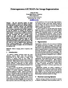
(2) where r(n, m) represents the original image and t(n, m) represents the segmented image, both of size [N, M ]. Table 5 shows the results of the segmentation and M SE and Snr for each of these segmentations. Inspecting Table 5 it is observed that for all images, even though the distance measure and the number of clusters were same, the mean square error was lower and correspondingly signal to noise ratio was higher when the extended pixel representation was used. It can be seen that the results look very similar to the original image because the clusters are colored with the mean color of all the pixels in that cluster. It can also be observed that the difference in results when the extended pixel representation is used is higher for images of low contrast. The extended pixel representation also performs better for pictures with high texture content. The smaller changes in color values of the pixels are separated and recognized better in extended pixel representations. Irrespective of the color space used, the extended pixel representation gives lower mean squared error and higher signal to noise ratio than the standard pixel representation for all images. All pixels that are similar in color get clustered into one segment which might represent a particular structure in the image. Thus, this representation adds more meaning to the image.

Conclusion The segmentation problem considered in this paper can be addressed by using the extended pixel representations.

65

Deeptha Girish et al.

MAICS 2016

pp. 63–67

Table 5: Results on segmentation of six images, using each of the three color spaces separately (2nd row), extended pixel representation (3rd row), and all three color spaces (4th row). Bold font indicates the smallest MSE.

`

a) Original Image

a) RGB Snr=35.3260db MSE=0.0050

a) RGB

RG

RG

GB

GB

BR

b) HSV Snr=54.8959db MSE = 0.0035

BR

Snr=39.3334db MSE=0.0033

a)

c) Original Image

b) Original Image

RGB HSV YCbCr Snr=37.4722db MSE=0.0173

b) HSV

HS

HS

SV

SV

c) YCbCr Snr=55.8133db MSE=0.0031

VH

VH

c) YCbCr

Snr=56.1241db MSE=0.0026

b) RGB HSV YCbCr Snr=57.064db MSE=0.0021

66

YCb

YCb

CbCr

CbCr

Snr=58.8801db MSE=0.0015

c)

RGB HSV YCbCr Snr=35.4811db MSE=0.0173

CrY

CrY

Deeptha Girish et al.

MAICS 2016

d) Original Image

e) Original Image

d) RGB Snr=47.4465db MSE=0.0014

d) RGB RG RG GB GB Snr=49.2535db MSE=0.0012

d) RGB HSV YCbCr Snr=48.1598db MSE=0.0013

pp. 63–67

f) Original Image

e) HSV Snr=44.0748db MSE=0.0062

BR

BR

e) HSV

HS

HS

SV

SV

VH

Snr=47.3483db MSE=0.0044

e) RGB HSV YCbCr Snr=26.9429db MSE=0.0038

67

f) YCbCr Snr=54.3042db MSE=0.00075

VH

f) YCbCr

YCb

YCb

CbCr

CbCr

CrY

Snr=54.9753db MSE=0.0007

e) RGB HSV YCbCr Snr=32.4912db MSE=0.0037

CrY