Fast Complex Adaptive Spline Neural Networks for Digital Signal Processing Aurelio Uncini, Fulvio Capparelli and Francesco Piazza Dipartimento
di Elettronica
e Automatica
- Universitd di Ancona Italy
Via Brecce Bianche, 60131 Ancona-Italy Fax: +39 (71) 2204464 - email: aurel@eealab. unian. it - Internet: http://nnsp.eealab.
Abstract ,
In this paper, we study the complex-domain arttficial neural networks called adaptive spline neural networks (ASNN), deflned in the complex domain, which are able to adapt their activation functions by varying the control points of a Catmull-Rom cubic spline. This kind of neural network can be implemented as a very simple structure able to improve the generalization capabilities using few training epochs. Due to its low architectural complexity this network can be used to cope with several nonlinear DSP problems at high sampling rate. In particular, we investigate the application of this new neural network model to the adaptive channel equalization problem. The goal is to design a receiver which compensates the HPA nonlinearities in digital radio links and performs the symbols extraction from the received data (demodulation process), when a 16-QA.M is used.
1. Introduction
R
The simplest solution we can imagine consists in involving gain a and slope b of the sigmoid a(l-e-‘x)/(l+e-br) in the learning process [I]. A different approach is based on the use of polynomial functions [2], which allows to reduce the size of the network and, in particular, the connection ’ This work is supported by the ((Minister0 dell’Universiti e della Ricerca Scientifica e Tecnologica>> of Italy
IEEE
complexity; in fact, the digital implementation of the activation function through a LUT (look-up-table) keeps the overall complexity under control. Drawbacks with this solution arise with the nonboundedness of the function (non-squashing) and with the adaptation of the coefficients in the learning phase. In [3] the direct adaptation of the LUT coefficients is proposed. This approach is characterized by a difficult learning process due to the large number of free parameters and the lack of smoothness of the neuron’s output. These are also the main reasons for the introduction of Hermite polynomials as substitutes for the so called supersmoother in the Projection Pursuit Learning approach of Hwang et al. [4]. Recently a new kind of artificial neural networks called adaptive spline neural networks (AWN) has been introduced [5-71. The adaptive activation function makes use of Catmull-Rom spline curve whose shape can be modified through some control points [8]. In particular in [7] this new architecture is presented in the context of the regularization theory: the authors demonstrate that ASNN embodies some regularity characteristics in its own activation function much better than the classical sigmoid can do .
ECENTLY’, a new interest in adaptive activation functions has arisen in the neural network community. In fact, such a strategy seems to provide better fitting properties with respect to classical architectures with sigmoidal neurons.
O-7803-4859- l/98 $10.0001998
unian.it/
903
The main advantages of this innovative structure, very useful for nonlinear adaptive signal processing, are: 1) the training sequence may be shorter than that required by the classical MLP; 2) the architecture is general and, unlike others approaches, it does not require a specific design; 3) the low hardware complexity (low overhead with respect to a simple adaptive linear combiner) makes it suitable for high speed data transmissions using a DSP device.
In particular, in this paper, we investigate the complex domain extension of the ASSN (CASSN) and the application of this new neural network model to the adaptive nonlinear channel equalization problem.
spaced along the x-axis (by a fixed step AX), FX,&) reduces to the first degree polynomial (3).
(2) 2. Complex Domain Functions (CASSN)
Spline-based
Activation C,ib)
2.1. Catmull-Rom implementation of the cubic activation function
l-
z&x
+
(3)
4x , i+l 1
0
It is worth-noting that fixing the values or qX reduces the total number of free parameters and the risk of overfitting.
Our idea consists in realizing a neuron with a more complex activation function than the sigmoid, able to reproduce the shape of a whole cubic spline along the directions specified by weights wj7 J 1
=
n.
Y
9***9
N
cpj(WjX)
= Cc,lWjX-~~13
j=l,...,n.
(1) 7
Referring to the papers [5-71 for further details, . . * .a* here we give some notes on such realization of an adaptive activation function. The goal is to give a global approximation using a structure as tractable as possible. In equation (1) we fmd a spline with N+l tracts: each of them is described by a different combination of the coefficients ci, because of the change in the sign of the kernels at aii. We have chosen to represent the activation functions through the concatenation of even more local spline basis functions, controlled by only four coefficients. As we want to keep the cubic characteristic, we have used a Catmull-Rom cubic spline. Using this type of spline we could exactly reproduce function (I), but, of course, this is not the cheapest solution, so we’ll take a different approach. .l
t
y
i=O
0
1I
1!
T
.....
i
1
I
4X.i
jt qX.i+l
qx.i+2 qx,i+J
%A’-3 qx,N-2 qx,N-I qx,N
i-th tract
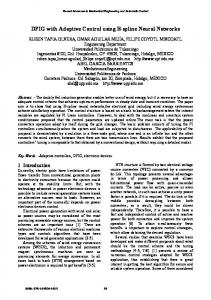
Figure 1. Control points of the Catmull-Rom spline based activation function: along the x-axis there is a fixed step k. The i-th tract starts with qX,i and ends with qX,i+3,but the controlled interval is only between qX,,i+land qX,i+2.
The qY coordinates are initialized by sampling a function like the sigmoid, which supplies the neural network with universal approximation capability. Along the x-axis, N+l points are taken; outside the sampling interval the neuron’s output will be held constant at the values qY,l, for the negative Xcoordinate, and &N-l for the positive X. In equation (3) the fixed step AX plays a rule of regularizing parameter (see [7] for more details).
of The activation function wi 11 be composed simpler cubic structures of local nature. The i-th tract is expressed by equation (2) where UE [0, l] and Q=(qx ,qY) (qx and qy are defined as control points). Such a spline interpolates the points Qi+l (~0) and Qj+z (~1) and has a continuous first derivative; the second derivative is not continuous only at the knots. Equation (2) represents a function if x-coordinates are ordered according to the rule qx,i < qx,i+l< qx,i+2C qx,i+3*The third degree equation Fxi(u)=xo, where ~0 is the activation of the neuron, gives the value of the local coordinate U: if the control points are uniformly
904
2.2 The Complex Function
Valued
Spline
Activation
The advantage of using complex-valued NNs instead of a real-valued NN counterpart fed with a pair of real values is well know [9- 121. In complexvalued neural networks one of the main problem to deal with, is the complex domain activation function, whose most suitable features have been suggested in [ 1 I]. Let F(S) be the complex activation function with SEC defined as the complex linear combiner output;
the main constraints that F(s) should satisfy are: 1) F(s) should be non linear and bounded; 2) in order to derive the backpropagation algorithm the partial derivatives of P’(S) should exist and be bounded; 3) because of the Liouville’s theorem F(s) should not be an analytic function.
where the symbol L=J is the floor operator. We find for each neuronj the local tract aj which sj belongs to, and the local coordinate uj. These expressions lead to neuron structure reported in Figure 2.
According to the previous properties, one possible choice, proposed in [ 121, [ 131, consists on the of real and imaginary activation superposition functions F(S’)=fRe(Re[SJ)+j~~(Im[~); where the functions fRe(a) and Am(*), can be simple real-valued sigmoids or more sophisticated adaptive functions.
2.3 The CASNN Learning Algorithm Following a development similar to [ 121, [ 131, for the synaptic weights, the learning algorithm is now extended to the spline’s control points.
Using a formalism similar to the one introduced in Widrow and Lehr in [14], and following a development similar to [9], [ 12- 131, for the synaptic weights, the learning algorithm is now extended to the spline’s control points.
IDk - X:‘)
l=M
A(/+t)w*(I+I) (m=l
nl
I= M-
mk
l,...,l
(5) with 0 I k I Nl and 0 I j I Nl+ The adaptation of the control points is ruled by r
=
(0 4 k7(,:‘)+,)R, [PI - 2k$e;‘c:‘1,R, @:“) /
; r
11
Figure 2. The complex-valued generalized sigmoid (GS) neuron structure (the structure of the imaginary part is omitted because it is identical to that of the real part).
Considering M total layers and indicating each of them with the index I, I= l,.. .,M, we can find the span ak and the local variable uk by Re[@ ]
(0 =kRe
=
N - 2 +-
h
2
(4
Im[$“]
(0 ‘kIm
The spline curve control points sampling a bipolar sigmoid (or activation functions); outside the the asymptotic shape of the sigmoid
(4a >
‘kRe
=
are initialized by other well-known sampling interval, is mantained.
N - 2 +-
=
2
Ax
3. Digital Radio Links Nonlinear Equalization
(4b) (0 ‘kIm
(6) where the patch index m=O, .. .. 3. The adaptation rates are pw for the connection weights and biases and p4 for the control points. The control point with index 0, 1, (N-l) and N are fixed.
(0 ‘kIrn
In microwave digital radio links, since on-board satellite power is a precious resource, to have an high the transmitter high-power amplifier efficiency, point: near the saturation operates (HW
(0 -
‘,I,
905
nonlinearities are introduced that can cause serious performance degradation of the received signal 1151.
baseband-equivalent system transmitter, HPA nonlinearity nonlinear system with memory.
(the cascade of and receiver) is a
It is well known that the 16 and 64 Quadrature Amplitude Modulation (QAM) links are very sensitive to nonlinear distortion, although they can exhibit better bit-error rate (BER) performance than equivalent phase-shift keying (PSK) systems on additive white noise Gaussian channels. The effects of the nonlinear channel with memory on the QAM signals are manifold, but three of them have particular importance: EXACT PHASE SHIFT (AM-PM) )/c-4&8)’
-6
---@
-8 LI”““““““““’ -8 -6
-4
-2
HPA INPUT POWER
0 (dB)
Figure 3. Typical traveling-wave memoryless input-output characteristic.
Transmitted symbols
STI M ~C(k)G(t-kr)
-
Pulse Shaping Filter
g(t)
40
~qk)dt - W A
tube
*
(TWT)
HPA
HPA
W)
Received symbols b(kT)
Figure 4. Block diagram of the digital radio link using a complex ASNN as nonlinea .r equalizer.
The nonlinearity of a typical HPA, a travelingwave tube (TWT) or a GaAs FET amplifier, affects both amplitude (AM/AM conversion) and phase (AM/PM conversion) of the amplified signal, and can be considered as memoryless, i.e. the HPA is a nonlinear system without memory under a wide range of operational conditions [ 161. In Figure 3 the AM-AM and AM-PM characteristics of a typical IHPA is reported. However, in practice, the a pulse shaping circuit transmitter contains (modulator) at the baseband or at the intermediate frequency (IF) stage virtually in all digital radio systems (see Figure 4). Therefore, the overall
Spectral spreading. The spectrum of the amplified signal after the HPA is much wider than the one of the signal before the HPA ; Intersymbol interference (ISI). Since the overall system has memory, each symbol of the QAM alphabet, usually referred to as a constellation point, becomes at the receiver a cluster of points due to the interference among symbols at the sampling instants. Constellation warping. The respective centers of gravity of the clusters caused by the IS1 are no longer on a rectangular grid as in the original constellation. The block diagram of the radio link used in our experiments is depicted in Figure 3. The complex input data sequence D(k), represents the points of the QAM constellation. The function g(t) represents the modulator filter impulse response: in the simulation we use a squareroot of a raised-cosine having a roll-off factor a equal to 0.5, and the over-sampling factor 1Mis chosen equal to 3. The g(t) filter length is equal to 5A4 taps. The model for the HPA is described in [ 161, the inputoutput HPA (memoryless) response is described by the AM-AM response, represented by the module, and the AM-PM response represented by the phase. This description assumes, for convenience, that the maximum possible HPA input power Win=Iu(t)12 is equal to 1W, and the maximum
shift is @, = $ ,
which are typical values [ 151. In the simulations the transmission of QAM signals are considered and, for the sake of brevity, only the case of 16 QAM has been reported. The maximum input power to the HPA Wimm is very close to the saturation point, and fixed equal to -1 dB (see Figure 3). Three complex-valued
equalizers have been tested:
1. complex-valued
-10
linear combiner (Al 5-l); lOLog
2. complex-value standard multilayer network with one hidden layer composed sigmoid neurons and linear output (N15-10-l); 3. complex-valued ASNN composed complex GS neuron (S 15-l).
neural by 10
-5 Networks with 5 sigmoidal neurons /
-45/)
/Networks
I 500
Figure 5. Training error comparison of architectures neurons.
I 1000 epochs
with 5 GS neurons
I 1500
-25
-30
MSE
:,:/‘----
-20
by only one
The training set consists of 6144 (2048xA4) input samples, v(t)+@) in the scheme of Figure 3, corresponding to 2048 target QAM symbols. Since the neural network output are the QAM complex constellation points, the network performs also the conversion. down-sampling For each epoch, a different realization of white zero-mean Gaussian noise n(t) is added, to obtain a S/N equal to 20 dB.
LdBl -10
-15
1
2000
for the Back & Tsoi system: with the same number of hidden
During the learning phase, the S15 - 1 and Al5 - 1 networks are trained for 100 epochs, while, in order to reach a suitable convergence, the standard MLP N15 - 10A 1 is trained for lo4 epochs. Both adaptation rates p4 and ,u~ for the S15-1 are chosen to be equal to 0.001; the same value is used for the MLP N15 10-1, while for the adaptive linear combiner A15-1 - pWis equal to 0.0001. Several tests using different networks initialization weights have been carried out. Figure 5 shows the plot of the MSE expressed in dB vs. the training epochs for the three architectures. The N15 - 10- 1 x-axis scale must be multiplied by a factor of 100 for a total of lo4 epochs.
-35
-40
-451 8
I 9
I 10
1 11
I 12 S/N
I 13
1 14
# 15
I 16
(dB)
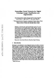
Figure 6. The symbols error probability (Pe) plotted vs. signal to noise ratio (S/N) at the input of the receiver using various equalization schemes.
In order to evaluate in a more realistic way the radio link performances, the symbol error probability (Pe) is computed. Figure 6 reports the Pe values vs. the S/N, both expressed in dB. From this figure we can observe that the proposed approach leads to significative improvements not only with respect to the classical linear adaptive filter, but also with respect to the already known sigmoid MLP based equalization technique.
4. Conclusions In this paper, a new complex domain architecture is proposed, based on an adaptive spline activation function approach, characterized by a limited complexity. In fact, the main problem using standard neural networks as nonlinear adaptive filters is the high degree of overall complexity, which accounts for a very long adaptation time and a high number of interconnections, that can hinder any practical application. This fact allows to overcome the previous drawbacks making possible to use effectively neural structures in real world problems. For what concerns the QAM equalization problem this advantage is even more evident, since the network reduces to a single complex neuron. Moreover, the reduced complexity is responsible for the shorter adaptation phase in terms of training epochs, as experimentally observed. Comparing our technique with classical linear approaches, we can notice that there is a low implementation overhead with respect to the adaptive linear filter, but with a significant improvement in the performance, both in terms of MSE (not reported in this paper) and symbol
907
error probability. As far as nonlinear methods are the proposed architecture exhibits concerned, performance comparable to finite-order inverse Volterra filters and to global compensation but with a much lower complexity that makes it suitable for an effective implementation.
PI
E. Catmull, R. Ram, ((A Class of Local Interpolating Splines)), in R. E. Barnhill, R. F. Riesenfeld (ed.), Computer Aided Geometric Design, Academic Press, NewYork, 1974, pp. 3 17-326.
PI
N. Benvenuto, M. Marchesi, F. Piazza and A. Uncini (
, Proc. of Intern. Conference on Neural Networks, ICANN91, Espoo, Finland, June 199 1.
References
PI
C. T. Chen, W. D. Chang, ((A Feedforward Neural Network with Function Shape Autotuning)), Neural Networks, Vo1.9, No 4, pp. 627-641, June 1996. F. Piazza, A. Uncini, M. Zenobi, c), in Proceedings of IJCNN, Beijing, Cina, pp. 11-343-349, Nov. 1992.
WI
H. Leung, S. Haykin, ((The Complex IEEE Trans Backpropagation Algorithnv,, Acoust. Speech and Signal Process, VolASSP39, pp.2101-2104, Sept. 1991. Cl11 S. Haykin, ((Adaptive Filter Theory)) Third Edition, Prentice Hall ed., 1996.
WI
N. Benvenuto, M. Marchesi, F. Piazza, A. Uncini, c>, in Proceedings of IJCNN, Nagoya, Japan, pp. II- 140 I- 1404, 1993.
PI
J-N Hwang, S-R Lay, M Maechler, R.D. Martin, J. Schimert, ((Regression Modeling in Back-Propagation and Projection Pursuit Learning)) IEEE Transactions on Neural Networks, 5(2), 342-353.
PI
S. Guarnieri, F. Piazza, Neural Networks with Activation Functions>) WCNN 95, Washington 1995.
A. Uncini,