Fast DRR generation for intensity-based 2D/3D image registration in radiotherapy D. Sarrut ∗,a,b S. Clippe b,a a laboratoire b Radiotherapy
LIRIS, Bˆ at L, Universit´e Lumi`ere Lyon 2, 5 av. Pierre Mend`es-France, 69676 Bron
departement, Centre de Lutte Contre le Cancer L´eon B´erard, 28 rue Laennec 69008, Lyon
Abstract Conformal radiotherapy requires accurate patient positioning according to a reference given by an initial 3D CT image. Patient setup is controlled with the help of portal images (PI), acquired just before patient treatment. To date, the comparison with the reference by physicians is mostly visual. Several automatic methods have been proposed, generally based on segmentation procedures. However, PI are of very low contrast, leading to segmentation inaccuracies. In the present study, we propose an intensity-based method, with no segmentation, associating two portal images and a 3D CT scan to estimate patient positioning. The process is a 3D optimization of a similarity measure in the space of rigid transformations. To avoid time-consuming DRRs (Digitally Reconstructed Radiographs) at each iteration, we used 2D transformations and sets of DRRs pre-generated from specific angles. Moreover, we propose a method for computing intensity-based similarity measures obtained from several couples of images. We used correlation coefficient, mutual information, pattern intensity and correlation ratio. Preliminary experiments, performed with simulated and real PIs, show good results with the correlation ratio and correlation coefficient (lower than 0.5 mm median RMS for tests with simulated PI and 1.8 mm with real PI). Key words: conformal radiotherapy, image registration, Digitally Reconstructed Radiographs, correlation ratio,
∗ Corresponding author. Email addresses:
[email protected] (D. Sarrut),
[email protected] (S. Clippe).
Preprint submitted to Elsevier Science
3 June 2003
1
Introduction
For more than one century radiation therapy has used X-rays to treat cancer. It has become one of the three main cancer treatment modalities, together with surgery and chemotherapy. To be efficient, radiation therapy must deliver a maximum dose of X-rays (now produced by linear accelerators) to the tumor while sparing surrounding normal tissue. Before the beginning of treatment, physicians and physicists have to establish a Radiotherapy Treatment Planning (RTP). The RTP defines the number of beams, their size, their shape, their tilt and the beam energy. This is now done in 3D with the help of a computed tomography (CT) scan of the patient. However, delivering X-ray doses is a fractionated process. For instance, at least 35 daily fractions are necessary to treat prostate cancer. But, installing the patient in exactly the same position every day is very difficult. This position is defined by the CT-scan used for establishing the RTP. Thus, the main difficulty is the day-to-day reproducibility of the patient setup. To check the positioning of the patient on the treatment couch, radiation therapists usually use only skin marks. For many years, displacements have been related. Mean setup errors are between 5.5 mm and 8 mm [1, 2, 3] with a maximum, though rarely reported, of 18 mm [4] or 16 mm [5]. Even in recent series, using of immobilization devices, displacements remain important: 22 % are between 5 and 10 mm [6] and 57 % are over 4 mm [7]. If setup errors have often been measured, their consequences have rarely been evaluated. Three studies have reported a degradation of the therapeutic ratio caused by discrepancies between the planned and the delivered treatment positions [8, 9, 10]. The first solution proposed to reduce setup errors and their potential serious consequences is patient immobilization. Immobilization devices such as polyurethan foam cast or thermoplastic mask have been developed. Numerous studies have shown their usefulness in reducing setup error rates [2, 3, 11, 12]. However they do not eliminate all errors and several recent series failed to show any improvement with the use of immobilization devices [13, 14]. The second solution to improve patient setup is called Portal Imaging, which is generally used as a complement of immobilization systems. Films acquired on the beam exit site of the patient allow the verification of patient position by comparing them with a reference image. Recently developed Electronic Portal Imaging Devices (EPID) have several advantages [15, 16, 17]. First, images are obtained immediately, unlike films which need to be processed. EPID thus allow on-line (immediate) setup error detection and correction. Secondly, EPID provide digital imaging, with image processing abilities. Fig2
ure 1 shows a schematic view of one type of EPID.
Accelerator device
Multi−leaf collimator
Patient
Treatment table Portal image device
Fig. 1. Electronic Portal Imaging Device (EPID).
Control images are used to detect and quantify setup errors relative to the planned position defined by a reference image. To date this detection has only consisted in a visual inspection by the physician. But this is inaccurate, labor intensive and time-consuming. Hence, there is a real need for tools to help physicians in this tedious task. Moreover, conformal radiotherapy adds reduced margins around the target volume. Therefore, acute patient positioning becomes essential to make sure that no target is missed, and minimize the risk of local recurrence. After setup error estimation, the aim of radiotherapists is to correct patient position before each treatment session. To that end, remotecontrolled treatment couches [18] and a tables with six degrees of freedom [19] can be used. In this paper, we propose to develop a fully 3D, automatic method for detecting setup errors in conformal radiotherapy. The paper is organized as follows. Section 2 is an overview of image registration techniques used in the context of patient positioning in radiation therapy. The general principles and notations are described in section 3. Section 4 describes the fast digitally reconstructed radiographs (DRR) generation. In section 5, we describe similarity measures used to compare DRR and PI. Section 6 presents experimental results, analysis and discussion. Finally, Section 7 concludes the paper. 3
2
Background
For several years, image registration methods used to determine patient position have compared portal images, which represent the real position of the patient on the treatment couch, and a reference image which represents the expected position. In this paper we focus on rigid transformations, assuming that the patient’s displacement is rigid. Methods are classified into two categories: feature-based methods using a segmentation step, and intensitybased with no segmentation step. Other criteria could be used, such as the different types of reference images: either simulator films, initial portal image validated by the physician, electronic portal images, or digitally reconstructed radiographs (DRRs). DRRs are 2D projection images [20]. They are computed with a specific volume-rendering from a CT-scan of the patient acquired before treatment which defines the reference position. Methods may either be 2D (three parameters to be determined: 2 translations and one rotation) or 3D (six parameters: 3 translations and 3 rotations). See also [21] for a review of setup verification in clinical practice.
2.1
Feature-based methods
Feature-based methods, using a segmentation step, are the most frequent methods used. Segmentation can be manual or automatic. In 1991, Bijhold et al. [22] presented one of the first methods of setup error measurement using portal images and a film as reference image. Image segmentation is done manually by delineating the bony outlines visible on both portal and reference images. Then, only the extracted, identical features are registered. Other methods use anatomical landmarks: three [23, 7] or five [24] homologous points determined in both images are matched. The main difficulty is the accurate definition of homologous points in the two images. The main drawback of these methods is that they generally only consider in-plane (2D) information, which is now known to be inaccurate in case of out-of-plane rotation or large translation [22, 25, 26, 27]. 3D methods were then developed. The first one uses several portal images taken from different projections [28, 23]. In this case, the registration is still 2D; it is performed independently with each PI, so it has the same drawbacks related beforehand. Marker-based methods of registration have also been developed [29, 30]. Radio-opaque markers are implanted in the body of the patient to overcome the problems induced by tumor movements. However the markers have to be fixed in the tumor volume itself, which is an important restriction for implantation. The second impediment of this method is the uneasy detection of these markers on very low contrast portal images. A fully 3D 4
method is proposed in [31, 32]. It is based on the registration of a 3D surface extracted from the CT scan with several image contours, segmented from the PI. Registration uses a least square optimization of the energy necessary to bring a set of projection lines (from camera to contour) tangent to the surface. Once structures have been extracted, the registration process is very quick. However it has never been experimented with real PI, which segmentation is much less accurate than with kilo-voltage radiographies. Fully 3D techniques could also require DRRs. One difficulty in this context is the computational time. Two methods are proposed. DRRs could either be computed at each step of the optimization process (on-line), but this must be very quick because the patient is awaiting on the treatment couch, or before the registration step (off-line), when there is no time constraint, each DRR corresponding to a known position of the patient. In 1996, Gilhuijs et al. [33, 34] developed a 3D method with partial DRR (computed with several selected points in the scanner) in order to speed-up the process. Murphy [35] also use partial DRR. The method was further evaluated by Remeijer et al. [27] in 2000: it is quick but limited by a high failure rate of the segmentation step in the portal images. It consequently requires human manual correction. To date, the segmentation step remains very difficult in PI because of their very low contrast, due to the high energy (5 - 20 Megavolt) of the X-rays used to acquire control images.
2.2 Intensity-based methods
A second class of methods uses the gray-level values of all the pixels in the images that must be compared. These methods assume that there is a statistical link between the pixel values of the images to be compared and that this link is maximum when the images are registered. For instance, Dong et al. [36] and Hristov et al. [37] used the linear correlation coefficient in a 2D method. They applied such measure to register portal images to modified DRRs (DRRs that have been filtered to resemble megavoltage images). Recently, a method using mutual information (MI) was proposed by Maes et al. [38] and Wells et al. [39]. It obtained interesting results in the context of multimodality image registration between PET, MRI and CT-scan. Other intensity-based similarity measures have been studied, such as the correlation ratio [40]. Preliminary studies on image registration using MI in the context of patient setup in radiotherapy have been published [41, 42, 43]. 5
3
Overview of the 2D/3D registration method
Considering published data and our preliminary works [41, 44], we decide to based our method on the following points: • No segmentation. PI are noisy images with low contrast for which accurate, robust and automatic segmentation is uneasy [27]. Intensity-based methods seems to be more suitable to compare DRR and PI, because, in this case, the accuracy of the final estimation is not related to the precision of the PI segmentation. Such methods are based on a similarity measure (see section 5), denoted S. • Use of several PI. Some patient displacements cannot be accurately evaluated from a single PI (typically, a translation along the viewing direction leads to very small image scaling). Thus, several PI must be acquired from different projections. We denote n the number of PI used simultaneously, I i the ith PI and P i the projection matrix associated with I i . Matrix P i is given by a calibration procedure. In practice, the number of PI is limited by the acquisition time and by the amount of radiation received by the patient, and two PI (n = 2), acquired from orthogonal projections, are used. However, our approach can be used with any n. i • DRR. The 3D CT scan is denoted V. We denote DU a DRR acquired aci cording to the projection P , for a given patient displacement denoted U : i DU = P i U (V). U is a rigid transformation matrix with 6 parameters (3 translations, 3 rotations). • 3D estimation. It has been shown that out-of-plane rotations lead to inaccurate or false estimations [26]. Thus, 3D methods are required. Hence, our approach consists in performing a 3D optimization over the search space defined by the type of the transformation (here only rigid transformations are studied). We denoted I the vector of n PI, and DU the vector of the n corresponding DRR. The similarity criterion is defined as a global similarity measure S in each pair of PI-DRR. ˆ = arg max S( DU , I ) U U
(1)
The optimization of eq. (1) is done with the Powell-Brent procedure described in [45]. • Combination of similarity. We propose in section 5.3 a way to define similarity between several pairs of images. • DRR pre-computation. At each iteration of eq. (1), there are n DRR generations and one evaluation of the similarity measure between n pairs of PI-DRR. However, DRR computation is a heavy task. Until now, most of the studies performing 3D estimation with DRR have focused on speeding up DRR generation [46, 33], but were detrimental to DRR quality (and thus to the quality of the similarity criterion). We propose here to replace the ex6
pensive DRR generation by another two-pass approach: pre-computed DRR and in-plane transformation. Such approach was also investigated in [47], but we propose here a mathematically justified decomposition.
4
Fast DRR generation
In order to overcome the expensive computational time of volume rendering, some authors [33] suggest that it is possible to generate a set of DRR computed according to a sampling of the search space before patient treatment. Such a step is only done once, before patient treatment (offline) and therefore does not have time constraints. However, the search space has six degreesof-freedom, and even with as few as ten points along each axis, it leads to a database of 106 DRR, which is not tractable in practice. However, we see in the next section that pre-computing DRR can be very useful.
4.1
Principle
The procedure relies on a precomputed set of DRR. During the optimization (eq. (1)), the generation of a DRR according to a given projection P1 is done in two steps: first, an adequate DRR is chosen in the set and then it is deformed according to a 2D affine transformation L. The next paragraphs shows how to choose the adequate out-of-plane DRR and how to compute L. Each image in the set of precomputed DRR is the projection of a rotation of the scanner, and this rotation is out-of-plane according to the optical axis of the initial projection, denoted P0 (the initial projection correspond to the projection of the portal image). Hence, such rotation has two degrees of freedom (see appendix F). The set of DRR is build by sampling the two parameters α, β. Out-of-plane rotations are bounded to a set of plausible rotations (±6◦ ) and sampled with a sampling step which allow sufficient accuracy (see experiments section 6).
4.2
Geometrical decomposition
Let P0 be the initial projection known by calibration process. Let P1 be the objective projection, corresponding to the DRR we want to generate. Parameterization is given in appendix A. Our goal is to find a projection Ph which is out-of-plane according to P0 , and a matrix L such that P1 ≈ LPh . To do this, we consider two intermediate projections P2 and P3 such that we know 7
how to build P2 from P1 , P3 from P2 and Ph from P3 . The figure 4.2 depicts the intermediate projections and their relationship in 2D (the optical center of projection Pi is denoted ci ).
c3 c1 = c 2
iso-center
P1
P0
c0 H P2
P3
F K
Fig. 2. Illustration in 2D of the projections (P0 , P1 , P2 , P3 ) and their optical centers (c0 , c1 = c2 , c3 ). Some 2D transformations (the rectification F and the scaling matrix K) are also depicted.
• We first consider the corrective rotation R and the projection P2 build as described in appendix B. The optical center c2 of P2 is the same that the 8
optical center c1 of P1 . Thus it exists a rectification matrix F such that F P2 = P1 (see appendix C). • Now, we consider the projection P3 (see appendix D), which has the same orientation than P2 . The difference between P2 and P3 is the distance between the optical center and the isocenter. We build a scaling matrix K (see appendix E), such that KP3 ≈ P2 . Note that if c1 is located on a sphere centered on the isocenter s, with radius kdk, we have c1 = c2 = c3 , K is the identity matrix and P3 = P2 . • The last step consists in using the out-of-plane/in-plane rotation decomposition described in appendix F in order to write P3 according to an outof-plane rotation of the initial P0 . We thus obtain P3 = C 0 Ph , with Ph an out-of-plane projection and C 0 an in-plane rotation matrix. Finally, we have: • Intermediate projection P2 is build from P1 by an in-plane rectification matrix F : P1 = F P2 • Intermediate projection P3 is build from P2 by an in-plane scaling matrix K : P2 ≈ KP3 • Out-of-plane projection Ph is build from P3 by the decomposition : P3 = C 0 Ph • Thus, we can write the objective projection as an in-plane affine transformation L of an out-of-plane projection Ph : P1 ≈ F KC 0 Ph = LPh
(2)
The computation of L and Ph only requires some vectors and matrices manipulations and has thus a negligible computational cost according to the remaining of the procedure. Moreover, applying the affine transformation L on a 2D image is straightforward and very fast. Finally, DRR generation (computation of L and Ph and application of L on a previously computed DRR) takes less than 20 milliseconds on a common 1.7Ghz PC.
5
Similarity measures
In the previous sections, we have advocated the use of intensity-based similarity measures to compare DRR and PIs. Such measures compare the relative position of two images. One image is the template image, denoted It , and the other one is the floating image If . In this paper, an intensity-based similarity measure S : It × If 7→ R is a criterion which quantifies some type of dependence between the intensity distributions of the images. It does not require any segmentation. The most widely known similarity measures are the correlation coefficient, entropy or mutual information [38, 39, 46]. In this section, 9
we describe the bases of these measures and discuss the choices that we have made.
5.1 Joint histograms
Joint histograms [38] are the underlying common base of most similarity measures used in image registration [48] (even if some measures do not require it, they can all be computed from joint histograms). This is a 2D histogram computed given a transformation U : we denote it HU . It is defined on the intensity distribution of the images (called Dt and Df ): HU : Dt × Df → R+ . HU (i, j) = nij is the number of points such as If (x) = j and It (T (x)) = i. Because of the discrete nature of images, T (x) does not generally coincide with a point of If , and an interpolation procedure must be applied. Probabilities pij must be estimated from quantities nij . Like most authors, we use a frequential estimation of the distributions: pij = nnij (where n is the number of points in the overlapping part of the images). Joint histogram is thus a contingency table and criterion S measures some type of dependence between the two intensity distributions. According to the type of the dependence (e.g. linear, functional), the considered type of intensities (numerical or categorical), and the different diversity measures used (variance, entropy), several measures can be defined [48].
5.2
Choice of the similarity measure
Four measures have been studied: correlation coefficient and mutual information have already been used in the PI-DRR comparison; Pattern intensity was proposed by Penney et al. [46] for the registration of a 3D CT with a 2D fluoroscopy image; finally correlation ratio was proposed by Roche et al. [49]. The correlation coefficient (denoted SCC ) [36, 37], assumes that a linear relation exists between the images intensities and measures the strength of this relation. The mutual information (SM I ) [38, 50, 39] computes a distance to the independence case, by way of the relative Shannon’s entropy. SM I is maximal when a functional dependence exists between the intensities. The pattern intensity (SP I ) [46] measure the “smoothness” of the image difference Idif f = I − sJ for each pixel in a small neighborhood. It requires three parameters: σ (see eq.(6)), r which define the size of the neighborhood and s which is a scaling factor used to build Idif f . The goal of this measure is to enhance bony structure correspondence, but it was designed for DRR/fluoroscopy registration and not for DRR/PI. The correlation ratio [40] (denoted by SCR ) assumes a functional relation between the intensity distributions and measures 10
its strength by the way of a proportional reduction of variance. Eq. (3), (4), (5) P and (6) express the three measures (with the mean mI = i ipi , the variance P P 2 = p1j i (i − mI|j )2 pij ): σI2 = i (i − mI )2 pi , and the conditional variance σI|j
SCC (I, J) =
X X (i − mI )(j − mJ )
σI σJ XX pij SM I (I, J) = pij log pi pj i j i
SCR (I|J) = 1 − SP I (I, J) =
X x,y
pij
(3)
j
(4)
1 X 2 pj σI|j σI2 j
(5)
σ2 σ 2 + (Idif f (x, y) − Idif f (k, l))2 (k−x)2 +(l−y)2 )