Fast pattern matching with time-delay neural networks - Heiko Hoffmann

Fast pattern matching with time-delay neural networks Heiko Hoffmann, Michael D. Howard, and Michael J. Daily Abstract— We present a novel paradigm for pattern matching. Our method provides a means to search a continuous data stream for exact matches with a priori stored data sequences. At heart, we use a neural network with input and output layers and variable connections in between. The input layer has one neuron for each possible character or number in the data stream, and the output layer has one neuron for each stored pattern. The novelty of the network is that the delays of the connections from input to output layer are optimized to match the temporal occurrence of an input character within a stored sequence. Thus, the polychronous activation of input neurons results in activating an output neuron that indicates detection of a stored pattern. For data streams that have a large alphabet, the connectivity in our network is very sparse and the number of computational steps small: in this case, our method outperforms by a factor 2 deterministic finite state machines, which have been the state of the art for pattern matching for more than 30 years.

I. I NTRODUCTION Our goal is to improve the speed of pattern matching in digital data. Rapid search is needed in large data sets, like video and audio streams and internet traffic. For example, for intrusion detection in internet traffic, the state of the art is not fast enough to search for all known attack signatures at modern day internet router speeds. For exact pattern matching, previous approaches focused on finding a string in a text. If wildcards are not allowed, then the Boyer-Moore (BM) algorithm [1] implemented on a standard serial computer is still the state of the art [2]. Its worst case computational complexity per input character is O(1). With wildcards, however, BM needs to be modified and becomes inefficient. An alternative are finite state machines [3], [4], which can deal with wildcards in the query string. The deterministic finite automaton (DFA) computes only one state transition per input character; thus, its computational complexity is O(1). Theoretically, the speed is independent of pattern length and alphabet size [4]. A disadvantage of DFA is that it requires an additional cost for building the statetransition table, which shows the state transitions depending on the input character, in preparation for the search. A statetransition table must be computed for every stored pattern that is to be matched against an input stream. In this article, we present a new type of network that sets connection delays optimally for pattern matching. This paradigm is a shift from the common practice in which connection delays are either uniform across connections or set at random a priori (see liquid state machines [5]). Moreover, we optimized the network to allow fast computation. Apart Heiko Hoffmann, Michael D. Howard, and Michael J. Daily are with HRL Laboratories, LLC (email: {hhoffmann, mdhoward, mjdaily}@hrl.com). This work was supported by HRL Laboratories, LLC

from keeping the number of computations at a minimum, we further require only integer additions. Particularly, the advantage of our novel method is an improvement in recognition speed if the input characters come from a large set (large alphabet). Large alphabets are in use, e.g., in 16-Bit Unicode, image data, computational biology [6], and in languages like Chinese and Japanese. For alphabets with more than 1000 characters, we found empirically for an implementation on a serial computer a more than two-fold improvement of recognition speed over the state of the art. Moreover, our network is suitable to be implemented in neural hardware, which results in higher speeds compared to a serial-computer implementation. Compared to state of the art pattern matching methods (Boyer-Moore algorithm and deterministic finite automata), our method has two further advantages: it does not require an upfront computational cost to compute shift or statetransition tables, and it can recognize partially-completed patterns as well (as an option). The remainder of this article is organized as follows. Section II provides the background for string search and our network design. Section III explains our novel network design and presents its capabilities. Section IV describes our implementation of this network. Section V shows a comparison with other methods. Section VI demonstrates in simulation the advantage of our new method over the state of the art in pattern matching. Finally, Section VII concludes the article. II. BACKGROUND A. String searching algorithms String search algorithms find matches of query strings within a text or input stream. The naive approach is to align the whole query string with the text starting from the beginning of the text and match each character in the query string with the corresponding character in the text. Then, the query string is shifted by one character and the matching process is repeated. This approach will find all matches in the text. However, the computational complexity is O(kn), where k is query size and n is the text size (number of characters). A more efficient approach is to shift the query string by k characters if a character is encountered that is absent in the query pattern, since any intermediate shifts are guaranteed to result in a mismatch with the query. This strategy is implemented in the Boyer Moore algorithm, which is still the gold standard for exact string matching without wildcards. The average computational complexity is O(n/k) if the alphabet is sufficiently large, and the worst case computational

complexity is O(n). However, the shift strategy fails if the query string contains wildcards. For patterns with wildcards, currently, the state of the art are deterministic finite automata, particularly, the AhoCorasick string matching algorithm [7], which is O(n). This algorithm has been the standard method for more than 30 years. Finite automata search for strings by transitioning between states; this transition is regulated by the current input character. As preparation, a query string must be converted into a state machine, which can be time consuming. The Aho-Corasick algorithm extends the idea of finite automata to building a state machine that can search through several query patterns simultaneously.

we will use integer delays. To illustrate the delays between neurons graphically, we reproduce all neurons for each time step (Fig 1). In the resulting plot, we can show a connection and its delay with a single arrow. Our network is defined through its neurons, the connections between them, and the delays for each connection.

B. Related work in neural networks Formally, our novel network is a special case of time-delay neural networks (TDNN) [8]. TDNNs are, however, conceptually different; instead of setting delays, in a TDNN the weight matrix of neural connections is expanded to include connections from previous time steps. Another instantiation of using delayed input can be found in recurrent neural networks, as, e.g., in the Elman network [9], which keeps a memory of previous hidden states. In the context of recurrent networks, Izhikevich introduced the concept of polychronization [10]. That is, time-shifted instead of simultaneous firing is critical for activating receiving neurons, because in real networks connection delays are heterogeneous. In general, several neurons may be activated by a time-shifted input pattern, and these neurons were called a polychronous group. Izhikevich demonstrated the phenomenon of polychronization in neural networks of spiking neurons that were described with several differential equations. Later, Paugam et al demonstrated a supervised learning approach to classify temporal patterns using a polychronous network [11]. For this classification, the authors learned the delays between a layer of recurrently connected neurons and an output layer. This work is one of the few where delays were learned and not just set a priori. All of the above neural models are computationally expensive. As a simpler alternative, Maier et al introduced the “minimal model” [12], which could exhibit polychronous activity without the complications of integrating differential equations. Our network is based on the neuron model from this minimal model.

Fig. 1. A neural network is represented in a time-evolution diagram to graphically show connection delays. The figure shows an example of a twotime-step delay between neurons 1 and 2. The time-evolution diagram shows temporal connections between neurons (Y axis) at different time steps (X axis).

B. Polychronous activation We use a simple integrate and fire neural model. If a neuron fires, it sends a spike with value +1 through all its outgoing connections. This spike is present only at a specific time step. Delayed through the connections, the spikes arrive at various time points at the receiving neurons. All incoming spikes that arrive at a receiving neuron at each time step are integrated and result at an activation level, a, which equals the number of incoming spikes at the specific time step, X a(t) = si (t − ∆ti ) , (1) i

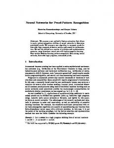
where si is either 1 or 0 depending on the activity of the transmitting neuron i, and ∆ti is the connection delay. If this activation level reaches a threshold, the receiving neuron fires. Each neuron may have its own threshold value. The delays may vary between connections. Thus, to activate a receiving neuron, the transmitting neurons should fire asynchronously; they need to fire in a specific sequence that matches the delays in the connections (Fig. 2). Izhikevich termed this property polychronous activation [10].

III. S ETTING DELAYS FOR PATTERN MATCHING We introduce the first network in which delays are set to achieve exact pattern matching. Here, a pattern is a time series of neural activations. The following sections describe the graphic illustration of connection delays, polychronous activation, pattern storage and recall, storing multiple patterns, absence of false positives, partially complete patterns, and wildcards. A. Connection delays Central to our approach is the setting of connection delays to achieve desired network functions. Throughout this article,

Fig. 2. Illustration of synchronous incoming spikes at the receiving output neuron (#4) when neurons 1 and 2 are activated in turn. Arrows show delayed transmissions through the neural connections.

C. Pattern storage and recall To store a string of characters, we represent it as a time sequence of neural activations. Each character corresponds to an input neuron. Thus, the pattern is given as P = {(s1 , t1 ), (s2 , t2 ), ..., (sk , tk )} ,

(2)

complexity. Figure 5 shows an example of storing a pattern with a single character wildcard “?”. Such a wildcard is simply represented as a time gap, i.e., extra delays for the connections. For storing consecutive “?” wildcards, i.e., wildcards of a given length, the delays can be adjusted accordingly.

where si is the input neuron, ti the time of activation of this neuron, and k the number of characters in the pattern. To store this pattern, we first compute the time gap between each character in the pattern and the pattern’s last character, ∆ti = tk − ti ,

(3)

This time gap is then stored as a delay in the network for the connection between the corresponding input neuron and a new output neuron that is assigned for this pattern (Figure 3 and Figure 4). For each character, a new connection is formed. Multiple connections of variable delays are possible between two neurons. A connection is only created when a new pattern is stored. Thus, for large alphabets (many input neurons) the connectivity is sparse. Apart from building connections, we set the threshold of the output neuron equal to the pattern size k.

Fig. 5. Example of storing a pattern with “?” wildcard (3, 2, ?, 1). Any neuron activated at time step 3 would be ignored.

D. Storing multiple patterns in one network Multiple patterns can be stored in the same network. For each new pattern, a new output neuron is created and the above storage procedure repeated. The network is capable of handling overlapping patterns, see Fig. 6 as an example. In recall, multiple patterns can be detected simultaneously.

Fig. 3. Example of storing the pattern (1, 2, 1) into the network. Three connections are added to the network.

This choice of neural delays and weights ensures that all occurrences of a pattern in an input stream are detected with the above operation and no false positives are obtained (see Section III-E). The flow for storing a pattern is shown in Fig. 4.

Fig. 6.

Example of delayed connections of two stored patterns

E. Uniqueness of the pattern recall

Fig. 4.

Process flow for storing a pattern.

A benefit of storing a string as delayed connections in our network is that wildcards of definite length are automatically taken care of, without increasing the computational

Our network detects all stored patterns in an input stream and does not produce any false positive, as we show below. Patterns of only a single character can be stored even though only two neurons are connected to each other (Fig. 7). Here, between the two neurons, multiple connections exist with different time delays. Lemma: Our network detects all occurrences of a pattern within an input stream without producing any false positive. Proof: By construction all occurrences of a pattern are detected. To prove that there are no false positives, we first note that the threshold for activation equals the number of connections to one output neuron. Moreover, one connection activates the output neuron only at one time step. Thus, all connections have to be active to activate the output neuron. To activate all connections the input neurons have to fire at

Fig. 7. Network connections and activations for a pattern that repeats a character multiple times, here (1, 1, 1). Multiple connections are formed between the same input and output neurons. However, only when the complete pattern is observed then the threshold for detection is reached.

the time points as specified in the stored pattern. Therefore, an output neuron cannot become active if less than the complete pattern is present. Thus, false positives are absent. F. Partially complete patterns The above method can be extended to detect partially complete patterns. Here, the threshold at an output neuron is reduced to a value smaller than k, allowing the network to detect partial matches with stored patterns. The value of the threshold regulates the completeness of the match. For example, if for a pattern of four characters a threshold of 2 is chosen, partial patterns are detected that consist of only two of the four characters that occur at the appropriate time points. This capability for partial matches allows us to apply our method to noisy patterns; noise in the input may activate the wrong neurons and therefore decrease the completeness of a pattern. G. Storing patterns with “*” wildcards As shown before, the network can deal with the “?” wildcard in a straight forward way. Including the multiplecharacter “*” wildcard, however, requires a slight modification. In this modification, we add an intermediate layer of neurons (Fig. 8), one neuron for each wildcard in a pattern. These intermediate neurons either project to another intermediate neuron if another wildcard is present or project onto the output neuron (dashed arrows show projections in Fig. 8). In both cases, the receiving neuron is activated over several time steps. Thus, this neuron remains in an excited state; i.e., only the remaining pattern is required to activate the neuron (see also Section IV). The threshold of an intermediate neuron equals the number of characters (not counting wildcards) up to the occurrence of the corresponding “*” wildcard. Thus, an intermediate neuron detects the partial pattern that is complete up to the “*” wildcard. When an intermediate neuron fires, it activates its receiving neuron by the same amount as the threshold of the intermediate neuron. Thus, the receiving neuron is

Fig. 8. Example for processing a pattern that includes a star wildcard (1, 4, ?, 2, *, 2). The partial pattern before the “*” projects onto an intermediate neuron (5), which in turn projects onto the output neuron. The intermediate neuron activates the output neuron over several time steps (dashed arrows).

excited equivalent to the reception of the partial pattern. An output neuron, as before, has a threshold equal to the size k of the complete pattern (not counting wildcards) and thus shows the same behavior as discussed before. Alternatively, as mentioned above, also here we could choose a lower threshold to allow detection of partially complete patterns. IV. I MPLEMENTATION To implement the network on a serial computer, we chose the following steps. First, we build lists of connections. For each neuron, we build an array for the connections. A new connection is added for each character in a pattern. Here, we need to store only those input neurons that are actually used in a pattern. The connectivity array contains for each connection the identification number of the target neuron and the delay. The number of connections per pattern equals the number k of characters in a pattern (not counting wildcards). Second, for the output neurons, we need to store a matrix that captures their activation over time: one dimension for the output neuron and one dimension for time. The stored patterns will have a maximum length (for the “*” wildcard we need to set a maximum length). Thus, we can make the time dimension of our matrix periodic, and the matrix size in this dimension is the maximum duration of a pattern, tmax . That is, at each time step t, the time dimension of the matrix covers the steps t to t + tmax − 1. The periodic boundaries require clearing the matrix contents to avoid spurious activations. After each input character is read into the network, the previous neural activations at time t are cleared, and then, t is incremented modulo tmax . As result, the space complexity (number of integer values) per stored pattern equals tmax for the activation matrix plus 2 times the average k for the connectivity array. In each computation cycle, an input neuron projects to all output neurons to which it is connected. For each connection, we need to look up the delay in the connectivity array. Using this delay, we shift to the corresponding entry in the activation matrix and increment this entry by 1. For the “*” wildcard, the intermediate neurons are part of the activation

matrix. If an intermediate neuron fires, it activates the row in the activation matrix that corresponds to the receiving neuron. The whole row is set to the value of the threshold of the intermediate neuron. All required operations are either integer additions or comparisons. Thus, our method can be implemented very efficiently. The estimated computational complexity per pattern and input character equals 1 + 3k/N additions, where N is the alphabet size. Here, k/N is the average number of connections per input neuron. For clearing the activation matrix, we need one addition, and for each connection, we need three additions: one to look up the delay, one to look up the entry in the activation matrix, and one to increment the entry in the activation matrix. On a serial computer, our method’s computation time is linear in the number of stored patterns. However, we could improve speed through parallelization, which could be done straightforwardly, e.g., by splitting patterns over different processors, by distributing output neurons, connections to these neurons, and their entries in the activation matrix. Since each processor requires only simple computations, this process is very suitable for graphics chips (GPUs). In addition, our network could be implemented on special neural hardware, reducing the cost of processing an input character to a single clock cycle. V. C OMPARISON WITH OTHER METHODS Our method has several advantages over the state of the art in string matching, which are deterministic finite automata (DFA) and the Boyer Moore algorithm, or their variants. These advantages are the inclusion of wildcards (“?” and “*”) without significantly increasing the computational complexity, the capability to detect partially complete patterns, and a high detection speed for large alphabets. To search for a single pattern, our method has a computational advantage over both DFA and Boyer Moore if the alphabet size is large. Figure 9 shows the parameter domains for which each method has an advantage over the other methods. This plot is based on the average computational complexity per input character and stored pattern. This complexity is O(k/N ) for our method, O(1/k) for Boyer Moore, and O(1) for DFA. When storing more patterns, the computational complexity of our method is worse than for the Aho-Chorasick algorithm, whose computational complexity is in principal invariant to the number of stored patterns. However, as mentioned above, we can gain speed through parallelization or implementation in neural hardware. Such implementations will likely not benefit deterministic finite automata. Parallelization does not improve the speed of Aho-Chorasick. A further disadvantage of DFA is that with increasing alphabet size, number of patterns, and inclusion of wildcards, the space complexity may explode, which leads to a sharp increase in computational time. Table I summarizes the comparison between our method and Aho-Chorasick.

Fig. 9. Parameter domains (in space of alphabet and pattern size) for which Boyer Moore (BM), deterministic finite automata (DFA), or our network have an advantage in computation speed. Boyer Moore cannot deal with wildcards; in that case, DFA is the only alternative. TABLE I C OMPARISON OF OUR NOVEL NETWORK WITH THE A HO -C HORASICK ALGORITHM FOR PATTERN MATCHING

Property Computational cost

Aho-Chorasick 2 additions per input character

Wildcards

Large increase in space complexity Does not improve above comp. cost High, especially if wildcards Not possible

Parallelization Comp. cost of pattern storage Detect partial patterns

Our network 1 + 3k/N additions per input character and stored pattern No significant additional cost Benefits storage of multiple patterns Low Possible

VI. S IMULATION R ESULTS We simulated our novel neural network to confirm its function and speed advantages. As test sets, we randomly generated input streams of one million characters and embedded 100 randomly generated patterns in each input stream at random locations. Our streams did include overlapping patterns. Each pattern contained five characters and had a total duration of ten time steps, i.e., contained five “?” wildcards. We generated ten of these input streams and tested on them a deterministic finite automata (DFA) and our novel method. As speed measure we evaluated the average computation time per stored pattern. We stored all 100 patterns that were distributed in the test sets into our network and build transition tables for the DFA for each pattern. Here, we ran 100 DFAs, i.e., 100 transition tables, in parallel. Thus, the obtained speed corresponds to the computational cost for searching for a single pattern (as in Table I). In measuring the speed of the search, we excluded any pre-processing stage like building a state-transition table for DFA (which highly depends on implementation). Including this pre-processing stage would be of disadvantage for DFA.

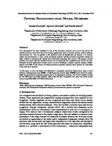
Our network did correctly detect all stored patterns within the input stream and did not produce any false positives. As for the speed, our novel method outperformed DFA for large alphabets (2x for alphabet size above 1000, see Fig. 10). For even larger alphabets, we found in our implementation of DFA that the computational time exploded, while with our novel network, the computational time stayed constant (here, we found a 10x improvement in speed for an alphabet size of two million). But the explosion of computational speed for DFA may depend on our implementation; therefore, we did not include it in our figure. This explosion does, however, demonstrate a common problem with state machines: they need to be sufficiently small to be efficient.

VII. C ONCLUSIONS We presented a novel paradigm for pattern matching. In contrast to prior work on neural networks, we set connection delays of a neural network to achieve a desired function. Herein, we exploited the property of polychronous firing for detecting a time sequence. As a result, we developed an algorithm that outperforms a 40-year-old established standard for pattern matching in the case of large alphabets. In addition, our method has several desired properties, particularly, the capability to deal with wildcards, to detect partially complete patterns, and to reduce the required computations to integer additions, i.e., no multiplications. The detection of partially complete patterns is beneficial if patterns are noisy, and a tolerance for detection is required. Since pattern matching is widespread, our novel method has the potential to find many applications, particularly, in areas like cybersecurity. Moreover, the paradigm of explicitly setting connection delays opens up new areas for algorithm development. R EFERENCES

Fig. 10. Comparison of the average computation time per pattern between our network and DFA. In each trial, we searched for all occurrences of a ten character string that includes five wildcards in a 1 Million character random text. The dashed curves show the theoretic values.

We compared our experimental results with our theoretical estimate of the computational cost (first row of Table I). To compare with the data, the cost values in the table were scaled such that the theoretical speed of Aho-Chorasick matched the average experimental speed of our DFA implementation. Experimental and theoretical results were in good agreement.

[1] R S Boyer, J S Moore, A fast string searching algorithm. Communications of the ACM, 20: 762-772, 1977. [2] M Zubair, F Wahab, I Hussain, M Ikram, Text scanning approach for exact string matching. International Conference on Networking and Information Technology, 2010. [3] A Gill, Introduction to the Theory of Finite-state Machines. McGrawHill, 1962. [4] M Sipser, Introduction to the Theory of Computation. PWS, Boston. ISBN 0-534-94728-X. Section 1.1: Finite Automata, pp. 31-47, 1997. [5] W Maass, T Natschlaeger, H Markram, Real-time computing without stable states: a new framework for neural computation based on perturbations. Neural Computation 14 (11): 2531-2560, 2002. [6] D Gusfield, Algorithms on Strings, Trees and Sequences: Computer Science and Computational Biology. Cambridge University Press, New York, USA, 1997. [7] A V Aho, M J Corasick, Efficient string matching: An aid to bibliographic search. Communications of the ACM, 18(6): 333-340, 1975. [8] A Waibel, T Hanazawa, G Hinton, K Shikano, K J Lang, Phoneme Recognition Using Time-Delay Neural Networks. IEEE Transactions on Acoustics, Speech, and Signal Processing, 37(3): 328-339, 1989. [9] J L Elman, Finding structure in time. Cognitive Science, 14(2): 179-211, 1990. [10] E M Izhikevich, Polychronization: Computation with spikes. Neural Computation, 18(2): 245-282, 2006. [11] H Paugam-Moisy, R Martinez, S Bengio, Delay learning and polychronization for reservoir computing. Neurocomputing, 71(7-9): 1143-1158, 2008. [12] W Maier, B Miller, A Minimal Model for the Study of Polychronous Groups. arXiv:0806.1070v1 [Condensed Matter. Disordered Systems and Neural Networks], 2008.