.
-.,,
Fast Query-Optimized Kernel Machine Classification Via Incremental Approximate Nearest Support Vectors Dennis DeCoste Jet Propulsion Laboratory
/
[email protected]
Caltech, 4800 Oak Grove Drive, Pasadena, CA 91109, USA
[email protected] .GOV Dominic Mazzoni Jet Propulsion Laboratory / Caltech, 4800 Oak Grove Drive, Pasadena, CA 91109, USA
Abstract Support vector machines (and other kernel machines) offer robust modern machine learning methods for nonlinear classification. However, relative to other alternatives (such as linear methods, decision trees and neural networks), they can be orders of magnitude slower at query-time. Unlike existing methods that attempt to speedup querytime, such as reduced set compression (e.g. (Burges, 1996)) and anytime bounding (e.g. (DeCoste, 2002), we propose a new and efficient approach based on treating the kernel machine classifier as a special form of k nearest-neighbor. Our approach improves upon a traditional k-NN by determining at query-time a good k for each query, based on pre-query analysis guided by the original robust kernel machine. We demonstrate effectiveness on high-dimensional benchmark MNIST data, observing a greater than 100fold reduction in the number of SVs required per query (amortized over all 45 pairwise MNIST digit classifiers), with no extra test errors (in fact, it happens to make 4 fewer).
1. Introduction Kernel machine (KM) methods, such as support vector machines (SVMs) and kernel Fischer discrmininants (KFDs), have become promising and popular methods in modern machine learning research (Scholkopf & Smola, 2002). Using representations which scale only linearly in the number of training examples, while (implicitly) exploring large nonlinear (kernelized) feature spaces (that are exponentially larger than the original
input dimensionality), KMs elegantly and practically overcome the classic “curse of dimensionality”. However, the tradeoff for this power is that a KM’s query-time complexity scales linearly with the number of training examples, making KMs often orders of magnitude more expensive at query-time than other popular machine learning alternatives (such as decision trees and neural networks). For example, an SVM recently achieved the lowest error rates on the MNIST (LeCun, 2000) benchmark digit recognition task (DeCoste & Scholkopf, 2002), but classifies much slower than the previous best (a neural network), due to digit recognizers having many (e.g. 20,000) support vectors. 1.1. The Goal: Proportionality to Difficulty
Despite the significant theoretical advantages of KMs, their heavy query-time costs are a serious obstacle to KMs becoming the practical method of choice, especially for the common case when the potential gains (in terms of reduced test error) are often relatively modest compared to that heavy cost. For example, it is not atypical in practice for a simple linear method to achieve 80-95% test accuracy, with a KM improving this by a few percentages more. Although such improvements are often significant and useful, it does raise serious “bang for buck” issues which hinder KMs from being more widely deployed, especially for tasks involving huge data sets (eg. data mining) and/or query-time constraints (e.g. embedded onboard resource-limited spacecraft or real-time robots). Also troubling is that KM costs are identical for each query, even for “easy” ones that alternatives (eg. decision trees) can classify much faster than harder ones. What would be ideal would be an approach that: 1)
Proceedings of the Twentieth International Conference o n Machine Learning (ICML-2003), Washington DC, 2003.
only uses a simple (e.g. linear) classifier for the (majority of) queries it is likely to correctly classify, 2) incurs the much heavier query-time cost of an exact KM only for those (relatively rare) queries for which such precision likely matters, and 3) otherwise, uses something in between (eg. an approximate KM), whose complexity is proportional to the difficulty of the query. 1.2. Summary of Our Approach The approach we propose in this paper directly attempts to find a good approximation to the above ideal. It is based on our empirical observation that one can often achieve the same classification as the exact KM by using only small fraction of the nearest support vectors (SVs) of a query. Whereas the exact KM output is a (weighted) sum over the kernel values between the query and the SVs, we will approximate it with a k nearest-neighbor (k-NN) classifier, whose output sums only over the (weighted) kernel values involving the k selected SVs. Before query-time we gather statistics about how misleading this k-NN can be (relative to the outputs of the exact KM, for a representative set of examples), for each possible k (from 1 to the total number of SVs). From these statistics we derive upper and lower thresholds for each step IC, identifying output levels for which our variant of k-NN already leans so strongly positively or negatively that a reversal in sign is unlikely, given the (weaker) SV neighbors still remaining. At query-time we then incrementally update each query’s partial output, stopping as soon as it exceeds the current step’s predetermined statistical thresholds. For the easy queries, early stopping can occur as early as step k = 1. For harder queries, stopping might not occur until nearly all SVs are touched.
scalar (C), a binary SVM classifier is trained by optimizing an n-by-1 weighting vector a to satisfy the Quadratic Programming (QP) dual form: minimize: Cyj=,aiajyiyj~(xi, xj)ai subject to: 0 5 ai 5 C , XEl cviyi = 0, where n is the number of training examples and yi is the label (+1 for positive example, -1 for negative) for the i-th d-dimensional training example (Xi).
+
xzl
The kernel avoids curse of dimensionality by implicitly projecting any two d-dimensional example vectors in input space (Xiand Xj) into feature space vectors (@(Xi) and @(Xj)), returning their dot product:
K(Xi,Xj) @(Xi). @(Xj).
(1)
Popular kernels (with parameters a, p , a) include: d linear: K(u,w) = 1‘ 1 * 21 UTW U&, polynomial: K ( u ,w) = (u. w a)P, 1 RBF: K ( u , v ) = e x P ( - s IIU - w1I2), normalized: K ( u ,w) := K ( u ,v ) K ( u ,u ) - i K ( v ,v)-i.
= +
The output f(z)on any query example z, for any KM with trained weighting vector p, is defined (for suitable scalar bias b also determined during training) as a simple dot product in kernel feature space:
f(z)= W * Q - b,
W=
n i=l
pi@(Xi),Q
a(.).
(2)
The exact KM output f(z)is computed via:
m
m
i= 1
i=l
f(z)= Cp,@(xi).@(z)-b = CpiK(xi,z)-b(3) For example, a binary SVM (of m support vectors (SVs)) has pi = yiai and classifies z as sign(f(z)).
3. Related Work on Lower Query Costs
A key empirical observation is that this approach can tolerate very approximate nearest-neighbor orderings. Specifically, in our experiments we project the SVs and query to the top few principal component dimensions and compute neighbor orderings in that subspace. This ensures that the overhead of the nearest neighbor computations are insignificant relative to the exact KM computation.
Early methods for reducing the query-time costs of KMs focussed on optimization methods to compress a KM’s SVs into a “reduced set” (Burges, 1996; Burges & Scholkopf, 1997; Scholkopf et al., 1998; Scholkopf et al., 1999). This involves approximating:
2. Kernel Machines Summary
by optimizing over all Zi E IRd and yi E 3 such that:
This section reviews key kernel machine terminology. For concreteness, but without loss of generality, we do so in terms of one common case (binary SVMs). Given a d-by-n data matrix (X), an n-by-1 labels vector (y), a kernel function ( K ) ,and a regularization
?(z) = W Q - b h
h
1
NN
f(x) = W . Q - b
i=l
(4)
(5)
‘Where the 2-norm is defined as IIu - v1I2 E u . u - 2u.
v + v . v and uT indicates the matrix transpose.
2Assume (without loss of generality) that only the first 5 n ) columns of X have non-zero pi.
m (for some m
minimizes the approximation cost:
yielding
nz nz F(x) = C y i s ( z i ) . 6 ( x ) - b = C y i K ( z i , x ) - b (7) i=l
i= 1
When small p M 0 can be achieved with nz > 1 kernel computations. Thus, (Romdhani et al., 2001) proposes a sequential approach, stopping early for a query as soon as its partial output drops below zero (indicating, in their application, a non-face).
A key problem with all such reduced set approaches is that they do not provide any guarantees or control concerning how much classification error might be introduced by such approximations. (DeCoste, 2002; DeCoste, 2003) develop sequential methods which quickly compute upper and lower bounds on what the KM output for a given query could potentially be, at each step IC. For classification tasks, these bounds allow one to confidently stop as soon as both bounds for a given query move to the same side of zero. However, computation of these bounds involves a IC2 term (due to the use of incomplete Cholesky decomposition). Despite working well over several test data sets, this overhead makes that bounding approach often useless for the sort of very high-dimensional image classification tasks we examine in our empirical work in this paper.
4. Nearest Support Vectors (NSV) The key intuition behind the new approach proposed in this paper is that, during incremental computation of the KM output for a query (via (3), one SV per step), once the partial KM output leans “strong enough” either positively or negatively, it will not be able to completely reverse course (i.e. change sign) as remaining p i K ( X i , x) terms are added. To encourage this to happen in as few steps as possible (for maximum speedup at query-time), we will intelligently (and efficiently) order the SVs for each query, so that the
largest terms tend to get added first. To enable us to know when a leaning is “strong enough” to “safely” stop early, we will gather statistics over representative data (before query-time), to see how strongly the partial output must lean at each step for such stopping to lead to the same classification (i.e. sign) as the exact KM output. That such an approach could work is not so surprising if one views the KM output computation (i.e. (3)) as a form of weighted nearest-neighbor voting, in which the p’s are the weights and the kernel values reflect (inverse) distances. Our inspiration is that small-k nearest-neighbor classifiers can often classify well, but that the best k will vary from query to query (especially near the discriminant border), prompting us to consider how to harness the robustness of a KM to guide determination of a good k for each query. Due to its relation to nearest-neighbors, we call our approach “nearest support vectors” (NSV). Let NSV’s distance-like scoring be defined as: NNscorei(z) =
K ( X i ,x).
(9)
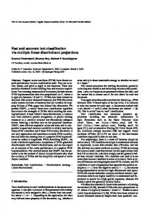
Figure 1 shows a positive query example (a “3” digit in a “8 vs 3” binary classification task using MNIST data), followed by its top 8 nearest SVs from the training set (those with largest ”score’s being first). The partial KM outputs (gk) for the first 8 steps using this SV ordering are shown above each SV. The two factors in the “score’s are shown in the first line of text under each SV (i.e. pi followed by the kernel value for the query and that SV). Not surprisingly, 3 of the first 4 nearest SVs are of the query’s class. More importantly, the p i K ( X i ,x) terms corresponding to the “score-ordered SVs tend to follow a steady (though somewhat noisy) “two steps forward, one step backward” progression, such that soon the remaining terms become too small to overcome any strong leanings. For example, the second four NSVs in Figure 1 already have considerable smaller PiK(Xi,x) than the first four. Encouraging and exploiting this phenomena is the key behind our approach. We will classify a query as soon as our pre-query worst-case estimates of how slow this drop off might occur indicate that a strong leaning is 3Actually, those kernel values are approximated during NSV ordering, to ensure nominal time costs, as described in Section 4.3. The exact kernel values (shown in Figure 1 below the approximate kernel values) are computed only as needed, as partial outputs are incrementally computed. Also, the KM bias term (b=0.0322 in this example) accounts for the first partial output (91)starting lower than the product of the first SV’s ,O and exact kernel value.
1.
4
0.148
0.99,0.275 -1.00,0.248 1.00,0.236 -1.00,0.215 0.59,0.322 -0.90,0.202 -0.78,0.231 0.125 0.102 0.129 0.086 0.054 0.012 0.098
Figure 1. Example of Nearest SVs.
unlikely to be reversed in sign, as the remaining (even lower scoring) NSVs are examined. Figure 2 summarizes our query-time algorithm. It trades off speedup ( m / k ) versus fidelity (likelihood of sign(g(z)) = sign(f(z))) by the choice of upper (Hk) and lower (Lk) thresholds, as the next section describes. Inputs: query x , SVs Xi, weights P i , bias b , and statistical thresholds (?&,Ilk). Output: g(x), an approximation of f(x). sort xi’s and pi’s by NNscorei(x);
g = -b; for k = 1 to m
9 = 9 if (g < end
+
Lk)
Pk
K(&,x);
or (g >
Hk)
(large 1st)
then stop;
Figure 2. Pseudo-code for query-time NSV classification.
4.1. Statistical Thresholds for NSV
We derive thresholds Lk and Hk by running the algorithm of Figure 2 over a large representative sample of pre-query data and gathering statistics concerning the partial outputs (g). A reasonable starting point is to include the entire training set X (not just the SVs) in this sample. Section 5.2 will discuss refinements.
Let gk(x) denote g(x) after k steps. A natural initial approach to thresholding (denoted Simple) is to compute Lk as the minimum value of gk(x) over all z such that gk(x) < 0 and f(x) > 0. This identifies Lk as the worst-case wrong-way leaning of any sample that the exact KM classifies as positive. Similarly, Hk is assigned the maximum g k ( x ) such that gk(x) > 0 and f(x) 0. When the query data is very similar to the training data, these Simple thresholds will often suffice to classify queries the same as the exact KM (but faster).
However, in practice, the test and training data distributions will not be identical. Therefore, we introduce a second method (denoted MaxSmoothed) which is based on outwardly adjusting the thresholds to conservatively account for some local variance in the extrema of the gk(2) around each step k. Specifically, we replace each Hk (Lk) with the maximum (minimum) of all threshold values over adjacent steps IC - w through k w. In our experiments in Section 6, we used a smoothing window of w=10. Our analysis suggests this was more conservative than required to avoid introducing test errors. However, experiments with narrower windows‘ (eg, w=2, giving slightly tighter thresholds) did not yield much additional speedups, suggesting that a moderate window size such as w=10 (relative to lOOO’s of SVs) is probably usually prudent. In any case, we assume that in practice an appropriate method of smoothing (e.g. choice of w) would be selected via some sort of prequery cross-validation process, to see what works best for a given task and data set.
+
4.2. “Tug of War”: Balancing SV+ vs SV-
Although the above approach suffices to provide some query speedups without introducing significant test errors, we have noticed that its speedups can be significantly suboptimal. This is because sorting NSVs solely by NNscorei(x) in the algorithm of Figure 2 leads to relatively wide and skewed thresholds whenever there is even a slight imbalance in the number of positive SVs (i.e. set SV+, with pi > 0) versus negative SVs (i.e. S V - , with pi < 0). For example, since an SVM constrains the sum of P over SV+ to be the same as that over S V - , the P values for the smaller set will be proportionally larger, making early (small k) leanings of gk(Z) tend towards the class with fewer SVs. This results in thresholds that are skewed and much larger than desired. In particular, we desire all but the earliest (strongest scoring) NSVs to effectively cancel each other, and thus make it unnecessary to explicit touch them during queries. However, such skewed leanings make that especially difficult to achieve. To overcome this problem, we replace the simple NSV
sort with an ordering we call “tug of war”. This involves adjusting the “score-based ordering so that the cumulative sums of the positive p and the negative /3 at each step k are as equal as possible. This often results in orderings which alternate between the top scoring positive and negative SVs, though not always - especially at later steps (large k ) , when ,f3 values are smaller and more widely varying. 4.3. Fast Approximate NSV Ordering
Metric (e.g. vp-trees, (Yianilos, 1998)) and spatial (e.g. kd-trees) indexing methods are often employed to avoid the expensive of full linear scans in nearestneighbor search. However, for the high-dimensional data targeted by this work, we find such indexing methods to often be practically useless. For example, the distribution of kernel distances using a degree 9 polynomial kernel on the MNIST data is so narrow that, for instance, triangular inequalities used by metric trees prune almost no neighbor candidates. That is, the minimum (non-zero) distance is greater than half the maximum distance, forcing full linear scans. Instead, we find that simple (though approximate) low-dimensional embeddings work much better on such data. Specifically, we do pre-query principal component analysis (PCA) on the matrix of SVs:
u s vT
=
x.
(10)
The k-dimensional embeddings of the SVs (pre-query) and the query x (during query) are given by projection:
X@) = V ( : 1 , : k)T
x,
z(k)
= V ( :1 , : k)T z. (11)
We use these small k-dimensional vectors, instead of the much larger original d-dimensional ones, to quickly compute (approximate) kernels and to approximately order NSVs for each Q as needed. When k