frequency domain, via the bispectrum (the polyspectrum associated with the ..... and gears); and (5) it can be implemented using relatively inexpensive computer ...
FAULT DIAGNOSTICS USING STATISTICAL CHANGE DETECTION IN THE BISPECTRAL DOMAIN
B. Eugene Parker, Jr., Hunter A. Ware, David P. Wipf, William R. Tompkins, Brian R. Clark, and Edward C. Larson BARRON ASSOCIATES, INC. 1160 Pepsi Place, Suite 300 Charlottesville, VA 22901 and H. Vincent Poor PRINCETON UNIVERSITY Department of Electrical Engineering Olden Street, Room B-210 Princeton, NJ 08544
1
ABSTRACT It is widely accepted that structural defects in rotating machinery components (e.g., bearing and gears) can be detected through monitoring of vibration and/or sound emissions. Traditional diagnostic vibration analysis attempts to match spectral lines with a priori known defect frequencies that are characteristic of the affected machinery components. Emphasis herein is on use of bispectral-based statistical change detection algorithms for machinery health monitoring. The bispectrum, a third-order statistic, helps identify pairs of phase-related spectral components, which is useful for fault detection and isolation. In particular, the bispectrum helps sort through the clutter of usual (second-order) vibration spectra to extract useful information associated with the health of particular components. Seeded and non-seeded helicopter gearbox fault results (CH-46E and CH-47D, respectively) show that bispectral algorithms can detect faults at the level of an individual components (i.e., gear or bearing). Fault isolation is implicit with detection based on characteristic a priori known defect frequencies. Important attributes of the bispectral SCD approach include: (1) it does not require a priori training data as is needed for traditional pattern-classifier-based approaches (and thereby avoids the significant time and cost investments necessary to obtain such data); (2) being based on higherorder moment-based energy detection, it requires few “simplifying” assumptions; (3) it is operatingregime independent (i.e., works across different operating conditions, flight regimes, torque levels, etc. without knowledge of same); (4) it can be used to isolate faults to the level of specific machinery components (e.g., bearings and gears); and (5) it can be implemented using relatively inexpensive computer hardware, since only low-frequency vibrations need to be processed. It thus represents a general methodology for the automated analysis of rotating machinery.
INTRODUCTION
It is widely accepted that structural defects in rotating machinery components (e.g., bearing and gears) can be detected through monitoring of vibration and/or sound emissions. Traditional diagnostic vibration analysis attempts to match spectral lines with a priori known defect frequencies that are characteristic of the affected machinery components. Short-term Fourier transforms, and related time-frequency 2
and time-scale techniques, are often used to detect non-stationary component failure signatures, which often result from the presence of a localized defect (e.g., bearing pitting or gear tooth fracture). The fact that typical component defects are localized spatially and have characteristic defect frequencies makes it possible to associate particular vibration patterns with specific machinery components. One of the major difficulties in machinery diagnostics is the problem of sorting through the enormous number of frequency lines present in vibration spectra to extract useful information associated with the health of a particular component. This is true even when phase-synchronous resampling of time-series vibration signals is performed to reduce the “smearing” of the frequency lines due to fluctuations in machine speed. Vibrational spectra in mechanical systems often contain bewildering mixtures of extraneous frequencies that provide little or no pertinent diagnostic information about the health of the machine. In rotating machinery applications, component characteristic defect frequencies generally occur as sideband modulations around the component carrier frequency (or harmonics thereof). In addition to such intra-component modulations, there are also inter-component modulations, such as a bearing defect modulating a gearmesh fundamental frequency and its harmonics. Disturbances due to localized component defects cause wideband impulses to be generated periodically at the characteristic defect frequency. These impulses, in turn, excite the component and its supporting structure, producing short-lived ringing signals of random amplitude. The strongest defect frequency is generally the one closest to the ringing mode. Since there is no reliable way of predicting the ringing modes of a component and its supporting structures, many potential defect frequencies must be monitored. Additionally, which ringing mode is dominant may depend on defect severity. The amplitude at the characteristic defect frequency often has such a low signal-to-noise ratio (SNR) that it will go unnoticed [1]. Power spectral analysis has long been applied to characterize and interpret vibrational signatures emanating from faults. However, this second-order technique has the serious drawback of discarding all phase information, which makes it virtually impossible to identify sets of signals that are phasecoupled. Higher-order statistics (HOS) and spectra furnish an effective and versatile mathematical approach for extracting information about such phase coupling. In particular, higher-order cumulants, and their associated Fourier transforms, known as polyspectra, exploit phase information. Such is not
3
true of second-order statistics (SOS) (i.e., the correlation function, which is the second-order cumulant). Since third- and higher-order cumulants vanish for purely Gaussian processes (such as the vibration spectra for defect-free gears and bearings), higher-order methods have the potential to increase the SNR in a large class of mechanical fault detection applications, such as those described herein. For example, the vibration of a normal bearing is Gaussian distributed [1]. The biggest drawback to the practical use of HOS is that such methods require longer data sequences than do SOS-based techniques in order to reduce the variance associated with the cumulant estimates. This is generally not a significant problem in machinery monitoring applications, however, because the rate at which faults develop is typically much slower than the rate at which relevant data can be acquired and analyzed. For machinery monitoring applications, HOS enable the analyst to discover phase-coupling effects among two or more spectral components of a process [1, 2]. The simplest type of such interaction is quadratic phase coupling between two frequency components, which is manifested by the presence of additional tones in the power spectrum at their sum and difference frequencies. It is noted, however, that the presence of sum and difference frequencies is a necessary, but not sufficient, condition for quadratic phase coupling. True phase coupling can be detected in the third-order cumulant sequence or, in the frequency domain, via the bispectrum (the polyspectrum associated with the third-order cumulant). As is shown below, the bispectrum furnishes a valuable means of detecting and characterizing nonlinear coupling effects in machinery [2]. In this paper, we introduce a technique for implementing bispectral analysis for use in machinery monitoring applications. Using phase-synchronous data, we illustrate how statistical change detection (SCD) in the bispectral domain can effectively detect and isolate faults in bearings and gears without reliance on substantial amounts of a priori data. With the SCD approach, we assume that the signal changes to be detected are manifested by the appearance of energy at certain a priori-known frequency pairs in the bispectral domain.\ This assumption is supported strongly both by the theory of defect\
With the SCD approach, there is little distinction between fault detection and fault isolation. Fault isolation is a natural
byproduct of successful fault detection since, in general, one does not simply detect a fault, but rather the bispectral energy that corresponds to a specific type of fault, among those types for which monitoring is being performed. Consequently, with the bispectral diagnostic technique, fault detection and isolation are united inextricably.
4
induced vibrations, as well as the demonstrated empirical findings of BAI and others (cf., [1, 2, 3]), which show that bispectra are effective in bearing and gear defect detection and sensitive to incipient (i.e., developing) faults. Application of these techniques to two different data sets (CH-47D and CH-46E helicopter transmission data) are presented herein.
QUICKEST DETECTION IN THE BISPECTRAL DOMAIN
In a recent paper [4], the authors derived a bispectrum-based quickest change detector, which was an extension of the analogous quickest detector based on the power spectrum. The power spectrum and bispectrum are defined respectively as e
K
u
(
> ;N �I ;N �I @
% �I� � I�
u
(
> ;N �I� ;N �I� ;N �I� � I� @ �
(
M;N �I M
�
3 �I
L
(1a)
e
where the superscripted asterisk denotes complex conjugation. In Eqs. (1),
(1b)
N
is an index denoting the
time block over which the Fourier coefficients of the accelerometer signal (denoted generically as are computed. The expectation operator, The power spectrum,
3 �I
(
;
)
, signifies an average over several such blocks.
, is a function of only one frequency; the bispectrum,
% �I� � I�
, on the
other hand, is a function of two independent frequencies.] It is noted, moreover, that the bispectrum, unlike the power spectrum, is complex-valued. Although the power spectrum can, for example, have tonal components at I� , I� , and I� � I� , the bispectrum is nonvanishing if and only if there is quadratic phase coupling among these frequencies. Eqs. (1) point to a means of generalizing the radiometric approach [5] that has been developed and applied in the second-order spectral domain to the bispectral domain. In problems of bearing and gear vibration monitoring [1, 2], the bispectrum has been shown to have zero mean under normal operating conditions, but non-zero mean in the presence of a defect. A natural approach to fault detection, therefore, is to test for a shift in the mean of % �I� � I� at particular frequency combinations. In this sense, the problem is very similar to the problem of detecting narrowband spectral energy, ]
Strictly speaking, the bispectrum involves coupling among three frequencies, I� � I� � and I�
5
u �� I
I�
.
which involves testing for a statistically significant increase in
3 �I
. By analogy, it is reasonable to
monitor for an increase in M% �I� � I� M. To compute time-varying estimates of 3 �I or % �I� � I� during the actual course of machinery operation, the ensemble averages in Eqs. (1) are computed over some trailing string of Fourier windows relative to a given time. Following are two possible approaches for extending the power spectral fault detection method to the bispectral domain. In the first approach, one appeals to a statistical model of ;N �I� ;N �I� ;
e N �I� � I�
approach is feasible because
M;N �I M
�
or
to derive a (locally) optimal test for a shift. In the spectral domain, this M;N �I M
�
is known, in the case of white noise, to be
� -distributed
with
two degrees of freedom. However, no such analogous statistical model for the bispectral case is known. An alternative approach is simply to extend SCD formulae that have been developed and applied in the spectral case to the bispectral domain. In the spectral domain, SCD techniques are less powerful than the model-based approach, and the same can generally be expected to be true in the bispectral case (once a statistical model for the distributional behavior of
e N �I� � I�
;N �I� ;N �I� ;
is developed).
However, the SCD approach should nonetheless be effective in detecting the appearance of significant bispectral energy at
�I� � I� �
In particular, the detection statistic
� 7opt �N
PD[ �xCxN
p p p E� p �N b C � � ORJ pp pp � E �
e
N ;
e
E� b E� ME� E� M
E�
E�
%pre-change
and
E�
(2)
M%P M
P C
was considered in [4]. Eq. (2) was obtained by replacing variances, with
�
�
and
�
, in the spectral case
, which respectively denote the pre- and post-change values of the bispectrum (i.e.,
and
E�
%post-change
). It is noted that
7opt
is a function of
�I� � I� ,
as well as the time, N .
The time, N , moreover, represents a relatively long time scale (various stages in the operating life of the machine), since long time spans are needed to compute averages over many Fourier windows. Since E� reflects the behavior of the machine under normal operating conditions, it can be interpreted as a known quantity (or one that can be estimated readily). However,
E�
is generally not known in
advance. It may be assumed, however, that E� is only slightly larger in modulus than E� , in which case
6
the appropriate detection statistic, in analogy with the spectral case [5], is the locally optimum one:
; N
7CR �N
PD[ �xCxN
�M%P M
b ME� M �
(3)
P C
Note that this detector depends only on E� . The threshold can be determined experimentally to control the mean time between false alarms. A potential concern about this methodology might be that it is too intensive computationally to be used in on-line applications. There are a few points that ameliorate this problem: (1) the ever-increasing computational throughput of digital signal processors; (2) the use of low-frequency vibrations (e.g., gearmesh fundamental and associated lower sidebands only) allows relatively low-frequency sampling to be used, reducing computational requirements; (3) the already limited (and further limitable) set of bispectral frequency pairs
�I� � I�
corresponding to characteristic defect frequencies at which the
bispectrum is computed; and (4) the generally slow onset of failures, which often permits non-real-time computation to be used (e.g., collect data, process data, collect data, etc.). Another issue concerning the bispectrum-based fault detection algorithm is its sensitivity to changes in absolute vibration level, such as occur with changes in operating (e.g., flight) regime. To address this concern, the bispectrum was normalized to obtain the magnitude-squared bicoherence function [1, 2]: �
M% �I� � I� M
p �I� � I�
� @ ( >M; �I M� @ �
( >M; �I� ; �I� M
�
(4)
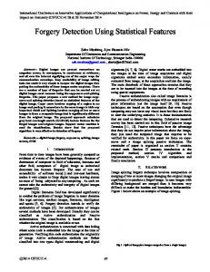
The bicoherence function is expected to be less sensitive to changes in vibration amplitude across varying operating regimes (e.g., torque levels). For example, Fig. 1, which is based on actual CH-46E helicopter data, illustrates the insensitivity to torque of the bicoherence function compared with the modulus of the bispectrum,
M% �I� � I� M
. In each graph, the abscissa represents the torque level (load
on the gearbox), whereas the ordinate represents the averaged and normalized[ bispectral signal values. The bicoherence exhibits no trend with respect to torque, whereas the bispectrum modulus declines dramatically with increasing torque. [
The largest averages computed using
p � I� � I �
and
M% �I� � I� M
were scaled proportionally.
7
, respectively, were scaled to unity, and other averages
Figure 1: Insensitivity of Bicoherence Function to Changes in Torque Level (CH-46E Dataset) The
7CR
statistic computed with the bicoherence function is then
; N
7CR �N
where
p�
PD[ �xCxN
represents the pre-change value of
P C
p �I� � I�
�pP
b
p� �
(5)
.
APPLICATION TO CH-47D DATA
A practical test of the performance of the
7CR
statistic in fault diagnostics was conducted using non-
seeded fault data from a CH-47D helicopter transmission in which a spiral bevel input pinion gear exhibits a classic tooth bending fatigue failure as a result of test cell overloading. The transmission was nominally fault-free at the start of the test. The data available consisted of two accelerometer recordings made simultaneously on the external gearbox housing (only one of which was used in the analyses herein), and a once-per-revolution tachometer signal corresponding to the shaft on which the gear that develops the tooth defect was mounted. The data were digitized at a sampling rate of 121,212 Hz and were available for 30-sec. of each minute over a total testing period of 23 min. 8
To correct for variations in shaft speed for the gear of interest, the original CH-47D time-series data were resampled to achieve phase-synchronous samples (see, e.g., [6, 7]). The resampled signal contained 310 samples per shaft revolution; since the spiral bevel input pinion shaft had 31 teeth, this corresponds to 10 samples per gear tooth. In computing the bicoherence function, Fourier windows covering 32 shaft revolutions (for a total of
��
d ��� = 9,920 samples) were used to compute the
;N �I
’s in Eqs. (1) and (4). The half-minute data segments contained an average of 184 Fourier
windows, which were ensemble averaged to obtain the bicoherence values used to compute the
7CR
statistics. The length of the Fourier windows determines the frequency resolution, frequency-domain data, which in this case is
Ishaft
��.
Ires
, of the resulting
Resampling greatly simplifies the interpre-
tation of the frequency bins obtained from a discrete Fourier transform. With the resampled data, shaft-revolution harmonics occur at every 32nd frequency line, i.e.,
��Ires , ��Ires ,
etc. Gearmesh har-
monics, which are 31 times higher in frequency, occur at every 992nd frequency line, i.e., �� ���Ires ,
etc. The sampling rate in the time domain determines the maximum frequency,
can be observed in the frequency domain, which in this case is To produce the bicoherence estimates, Igearmesh
. The
7CR
I�
was held fixed at
� �
d � ��� �
Igearmesh
Ires
, and
= I�
���Ires ,
INyquist
, that
�� ���Ires .
was swept from 0 to
results are displayed in Fig. 2, which plots time on one abscissa and
I�
on the other.
An end-on view of Fig. 2 (viewing the frequency axis end on) is provided in Fig. 3. There are two noteworthy results in these figures: 1. In Fig. 2, the large deviation from baseline, indicating a fault, is detectable approximately at time 16 min. This corroborates well with the findings of a post-failure metallurgical analysis that was performed, which suggests that a gear-tooth microcrack initiated at about 12 min. into the test. 2. In Fig. 3, which has twice the resolution on the frequency axis as Fig. 2 (i.e., every 16th rather than every 32nd spectral line is plotted), we see that the increase in the values of 7CR occur only at frequencies that are integer multiples of
Ishaft
, i.e., every other frequency line, which means
that bispectral energy resides largely in the gearmesh sidebands (whose spacing is equal to Ishaft ). 9
1
0.9
1
0.8
0.8
0.7
0.6
T
i
Ti
0.6
0.5
0.4 0.4 0.2 0.3 0 30
0.2 25 20
20 15
0.1
15 10
10 5
f1
0
5 0
0
5
10
15
20
25
30
f1
Time (min)
Figure 2: Isometric View of Time-Averaged
Figure 3: End-on View of Time-Averaged
Bicoherence-Based 7L (CH-47D
Bicoherence-Based 7L (CH-47D
Dataset)
Dataset)
The argument might be made that the sort of catastrophic failure resulting from an overload-induced fault could be detected using even the most rudimentary detection algorithm. Why, then, does one need the bispectral statistic? Fig. 4 depicts the accelerometer RMS signal vs. time for the duration of the CH-47D dataset. The non-seeded fault manifests itself at approximately time 20 min., in contrast to the bispectral approach, which detects the fault by time 16 min., an improvement of approximately 4 min. Although this seemingly small time savings may not appear to justify the bispectral methodology, in certain critical systems (e.g., helicopter gearboxes), it can make the difference between life and death, such as if it provides sufficient warning for executing a safe landing. Even in such critical applications, one still must remember that this test scenario effectively simulates an accelerated lifecycle of a helicopter transmission. In fact, the transmission is in an entirely different stage of wear at time 16 min. than at time 20 min., when the fault is much more obvious. Therefore, the 4-min. time interval is critical as it maps to a potentially much larger timeframe (possibly weeks or months) in the true life of a transmission. Early warning can provide the time needed to avoid catastrophic failure and to optimally schedule necessary maintenance activities, whether for helicopter or industrial applications.
10
280
270
RMS Signal Units
260
250
240
230
220
210
200
2
4
6
8
10
12 Time (min)
14
16
18
20
22
Figure 4: RMS Signal Strength vs. Time (CH-47D Dataset)
APPLICATION TO CH-46E DATA
As discussed earlier, different faults have different characteristic signatures. These signatures are scaled as a function of the parameters (i.e., bearing diameter, number of gear teeth, etc.) of the component under consideration and speed of the shaft on which the component resides. Such scaling permits a fault to be isolated (i.e., identified) down to the component level. This was demonstrated using CH-46E helicopter seeded-fault gearbox data that were collected on the Westland Helicopters Ltd. Universal Transmission Test Rig [8, 9]. The test rig was used to measure the diagnostic vibration of a CH-46E helicopter combiner transmission under eight different test conditions: (1) no defect, (2) planetary bearing corrosion, (3) spiral bevel input pinion bearing corrosion, (4) spiral bevel input pinion spalling, (5) helical input pinion chipping, (6) helical idler gear crack propagation, (7) collector gear crack propagation, and (8) quill shaft crack propagation. Data were collected at nine different input torque levels between 27% and 100% of maximum torque. Data were sampled originally at a rate of 103,116.08 Hz for a time interval of approximately 22.6 sec. for each test condition at a given torque level. Ten channels of data were recorded, which included eight accelerometers, a tachometer signal (which was fitted in place of the blade fold drive motor and provided 256 pulses-per-revolution with a once-per-revolution signal superimposed on it), and one sinusoidal reference tone.
11
As with the CH-47D data, the original CH-46E data were resampled to achieve phase-synchronous samples for each component of interest. In the case of the collector gear, for example, we utilized 32 samples/tooth, which, since the gear had 74 teeth, yields 2,368 samples/rev. In the case of the helical idler gear the numbers were 32 samples/tooth, for a gear with 72 teeth, yielding 2,304 samples/rev. A Fourier window 32 shaft revolutions long was employed in these analyses, as in the CH-47D analysis. Each data file contained 29 Fourier windows, which were ensemble averaged to obtain the bicoherence values. Since each of the files of the Westland dataset represents a distinct fault or no-fault case, it is not possible to demonstrate fault detection via the 7CR statistic. This is because the no-fault, pre-change background noise level will not be useful in the fault cases, since the transmission was disassembled between data collection episodes. This reemphasizes the need to establish, on-line, a background noise floor,
p�
, as indicated in Eq. (5).
Therefore, for purposes of demonstrating fault isolation at the component level on the Westland dataset, we used the average value of the power function in the denominator of Eq. (4), i.e., the quantity � @ ( >M; �I M� @, �
( >M; �I� ; �I� M
across the characteristic defect frequencies. This power function was
computed for the no-fault data file and for three different fault data files, namely: (1) collector gear crack propagation, (2) helical idler gear crack propagation, and (3) spiral bevel input pinion inner-race bearing defect. For each of the three faults and the no-fault case, results were compiled for torque levels of 70%, 80%, and 100% (the only torque settings that were available in all four cases). Fig. 5 illustrates the results for fault isolation using the aforementioned power function. In each histogram, the four bars represent the average of the power function for all the frequency pairs �I� � I� associated with a particular fault scenario. The three histograms in the left column of Fig. 5 were generated with
I�
set equal to the collector gearmesh frequency and
I�
to harmonics of the collector
gear revolution frequency. The vibration data used in these twelve runs were based on accelerometer #7, which was spatially closest in the gearbox to the collector gear. The center column of histograms was generated using the corresponding �I� � I� combinations associated with the helical idler gear. For these runs, accelerometer #3 was used since it was the one closest to the gear in question.
12
1
Collector Sampling 100% Torque
Normalized Power Function
0.5 0
1
1
1
2
3
4
Collector Sampling 80% Torque
0
1
1
2
3
4
Collector Sampling 70% Torque
0
1
1
2
3
4
Helical Sampling 80% Torque
2
3
4
0
Bearing Sampling 100% Torque
0
1
1
2
3
4
Bearing Sampling 80% Torque
0.5
1
2
3
4
Helical Sampling 70% Torque
0.5
1
1 0.5
0.5
0.5 0
Helical Sampling 100% Torque
0.5
0.5 0
1
0
1
1
2
3
4
Bearing Sampling 70% Torque
0.5
1
2
3
4
0 1
2
3
4
Histogram Key: 1 = Spiral Bevel Input Pinion Inner Race Fault 2 = Helical Idler Crack Propagation 3 = Collector Gear Crack 4 = No Fault
Figure 5: Fault Isolation Results for Westland Data The third column of histograms shows the results of the power function applied to a case involving a bearing fault. In particular, this was a spiral bevel input pinion bearing with an inner-race defect. Accelerometer #3 was monitored in this case as in the helical idler gear fault. For this bearing fault, I� was set equal to the bearing shaft frequency, and I� was set equal to Ires . From a diagnostics
viewpoint, bearings are different from gears. For example, they have more characteristic frequencies, and the rolling elements internally have an appreciable amount of “slip” freedom. The extent of sliding motion, for example, depends on torque level, shaft speed, and lubrication. Hence, the defect frequencies (e.g., inner or outer ball-pass frequency) that are actually observed are not as rigidly linked to the shaft frequency as they are in gear defects. The important result from Fig. 5 is that in all cases, the type of fault that actually occurred is identified correctly; i.e., the power function corresponding to the actual defect (frequencies) is always the largest. This demonstrates that faults can be isolated successfully at the component level with this approach.
13
CONCLUSIONS
The investigations that were presented are based on the notion that changes in bearing and gear health are manifested by the appearance of energy at certain identifiable frequency pairs in the bispectral domain. Through proper selection of these pairs, one can discriminate among different potential fault sources to pinpoint the faulted component. Research in this direction is motivated by the interest in monitoring machinery components (e.g., bearings and gears) for structural failures. Bispectral-based diagnostic techniques were introduced and tested on two different helicopter transmissions. The results are promising and demonstrate the feasibility of bispectrum-based statistics for machinery monitoring applications. Bispectral information is especially useful because the requirement of phase coupling among particular frequency combinations greatly reduces the overwhelming clutter of frequency lines in the power spectrum. Moreover, such coupling is most pronounced in the presence of machinery faults, not under normal operating conditions. The bicoherence function reduces the variation in the bispectrum across different torque levels and loads. Restricting attention to certain frequency pairs facilitates isolation of effects (e.g., sideband tones) that are related to the defect frequencies of given components. Important attributes of the bispectral SCD approach include: (1) it does not require a priori training data as is needed for traditional pattern-classifier-based approaches (and thereby avoids the significant time and cost investments necessary to obtain such data); (2) being based on higher-order moment-based energy detection, it requires few “simplifying” assumptions; (3) it is operating-regime independent (i.e., works across different operating conditions, flight regimes, torque levels, etc. without knowledge of same); (4) it can be used to isolate faults to the level of specific machinery components (e.g., bearings and gears); and (5) it can be implemented using relatively inexpensive computer hardware, since only low-frequency vibrations need to be processed. It thus represents a general methodology for the automated analysis of rotating machinery.
14
REFERENCES [1] C.J. Li, J. Ma, and B. Hwang 1995 Transactions of the ASME, Journal of Engineering for Industry 117, 625-629. Bearing localized defect detection by bicoherence analysis of vibrations. [2] J. Jong, J. Jones, P. Jones, T. Nesman, T. Zoladz, and T. Coffin 1994 Proc. of the 48th Meeting of the Mechanical Failures Prevention Group: Advanced Materials and Process Technology for Mechanical Failure Prevention, 379-389. Nonlinear correlation analysis for rocket engine turbomachinery vibration diagnostics. Willowbrook, IL: Vibration Institute. [3] T. Zoladz, E. Earhart, and T. Fiorucci 1995 Marshall Space Flight Research Center, NASA Technical Memorandum 108491, Bearing Defect Signature Analysis Using Advanced Nonlinear Signal Analysis in a Controlled Environment. [4] B.E. Parker, Jr., H.V. Poor, E.C. Larson, T.A. Hamilton, and J.P. Frankel 1997 NOISE-CON ’97, 319-324. Statistical change detection using nonlinear models. [5] H.V. Poor 1994 An Introduction to Signal Detection and Estimation. (New York: Springer Verlag). [6] J. Jong, J. McBride, J. Jones, T. Fiorucci, and T. Zoladz 1996 Proceedings of the 50th Meeting of the Society for Machinery Failure Prevention Technology: Technology Showcase – Integrated Monitoring, Diagnostics, and Failure Prevention, 441-451. Synchronous phase averaging method for machinery diagnostics. Willowbrook, IL: Vibration Institute. [7] G.P.
Succi,
1995
Proceedings of the 49th Meeting of the Society for Machinery Failure
Prevention Technology: Life Extension of Aging Machinery and Structures,
pp.
113-115.
Willowbrook, IL: Vibration Institute. [8] 1993 Westland Helicopters Ltd. Research Paper RP907, Final Report on CH-46 Aft Transmission Seeded Fault Testing, Vols. 1 and 2. [9] 1994 Westland Helicopters Ltd. Mechanical Research Report MRR20168. CH-46 Aft Transmission Seeded-Fault Testing Analysis of Vibration Recordings. (DTIC Document Number AD-B180 276).
15
ACKNOWLEDGMENTS
This investigation was funded by the Office of Naval Research (ONR) under Grant No. N0001496-1-1147 (Subrecipient Agreement No. S96-8) and Contract N00014-95-C-0413. The authors thank Dr. Thomas M. McKenna of ONR and Mr. G. William Nickerson of the Pennsylvania State University Applied Research Laboratory for their support of this work.
16