feature selection for tool wear diagnosis using soft ... - CiteSeerX

Proceedings of the ASME, Manufacturing in Engineering Division, (MED-Vol.11), pp. 157-163, 2000

FEATURE SELECTION FOR TOOL WEAR DIAGNOSIS USING SOFT COMPUTING TECHNIQUES

Kai Goebel GE Corporate R&D Niskayuna, NY 12309 [email protected]

ABSTRACT – This paper examines feature selection methods in the context of milling machine tool wear diagnosis. Given raw sensor signals acquired during experiments, a pool of features was created through calculation by several feature extraction methods. Five techniques for selecting the most discriminating features were employed. These techniques included decision trees, neuralfuzzy methods, scatter matrix, and a crosscorrelation method. We used a diagnostic neural network to evaluate the five different feature selection schemes by comparing their classification rate and test errors. Keywords: feature selection, feature extraction, machining, diagnosis, sensor fusion, soft computing

1. INTRODUCTION Feature subset selection is the process of choosing particular elements from a given set of candidate features. To achieve desired performance of any diagnostic algorithm, it is necessary to pick the most relevant features as inputs to the algorithms from the multiple sensor data and calculated characteristics. The feature selection process can not only reduce the cost of recognition by reducing the number of features that need to be collected, but also improve the classification accuracy of the system. The purpose of the process is to optimize the classification ability based on training data and to predict future cases. This implies that there is one or more sets of features with which this diagnostic task can be performed better than with others. The selection process is not necessarily trivial. There is an overwhelming number of features one could create from raw data. Using all possible features is not practical because irrelevant features add noise to the classifier making the diagnostic task harder or impossible or computationally prohibitively expensive. Choosing even from a moderately sized set of features is often times based on individuals’ experience and some heuristics. Based on the diagnostic task and

Weizhong Yan GE Power Systems Schenectady, NY 12345 [email protected]

model at hand, traditional methods do not always lead to the best feature set. In this paper, we address which feature selection approaches can select the most important features in a quick and effective manner and use techniques from Soft Computing for this purpose. Five different feature selection schemes were employed and compared. The five schemes rate the features based on their discriminating power. The three top ranked features of each scheme were chosen and fed into a diagnostic neural network for evaluation. The performance of the five schemes were evaluated by comparing both classification rates and the error of an evaluation function. The reminder of the paper is organized as follows. Section 2 gives background information about feature selection methods. Details of the five feature selection schemes are outlined in Section 3. Section 4 describes the experimental setup. The feature extraction process is laid out in Section 5. Results of the application to the tool wear diagnosis problem and conclusions are presented in Sections 6 and 7, respectively. 2. BACKGROUND Feature selection has been widely studied and documented for example by Kira [1] in 1992 and Dash [2] in 1997 who carried out comprehensive overviews of feature selection techniques. Feature selection methods can be viewed from three different angles: (a) which search method is employed; (b) what evaluation criteria are used; (c) and which real-world applications are the feature selection exercised with. These aspects are here briefly illuminated. a) Search methods – Depending on which search method is used, feature selection methods can be categorized into (i) optimal search (exhaustive search [3] and branch & bound algorithms [4]), (ii) heuristic search (sequential selection [5], floating

selection [6], and decision tree methods [7]), (iii) random search (genetic algorithms [8], simulated annealing [9], and Bayesian network algorithm [10]), (iv) and weight based search (fuzzy set theory [11], fuzzy feature selection [12], neural networks [14, 15], neuro-fuzzy approach [13], and relief [2]). Compared to random search and weight based search, optimal search is more computationally expensive and therefore sometimes not feasible. b) Evaluation criteria - Each search method of feature selection has to use evaluation criteria to measure the “goodness” of a particular subset of features which helps in the selection process. Widely used evaluation criteria include (a) distance based measures, such as Mahalanobis distance [16], Hausdorff distance [17], and metric approach [18]; (b) entropy measures [19, 20]; (c) statistical measures [16, 20]; (d) correlation based heuristic measures [21]; e) accuracy measures [22]; and (f) relevance measures [23]. With regard to how to implement the evaluation criteria, filter and wrapper are the two well-known approaches [24]. The filter approach selects features as a result of preprocessing based on properties of the data itself independently of the learning algorithm. The wrapper approach, on the other hand, uses the learning algorithm as part of the evaluation. Typically, the wrapper approach gives more accurate results, but is also computationally more expensive. Hybrid approaches that combine filter and wrapper approaches have also been proposed [25]. c) Real-world applications - Feature selection is a crucial element for applications in areas such as statistics [26], pattern recognition [5, 27], machine learning [22, 24, 28], and data mining [29, 30]. Of particular interest to us are machine-tool condition monitoring and tool wear diagnosis. These are critical tasks for every machining operation, especially for unattended and automated machining. While most research work focuses on developing diagnostic algorithms for machine condition monitoring, not much attention has been paid to selecting features for improving the performance of diagnosis [31, 32]. In Jack’s [31] study, genetic algorithms were used to select the most significant features as inputs to a neural network. Pan [32], on the other hand, proposed using a fuzzy cluster feature filter to remove redundant signal features.

3. FEATURE SELECTION SCHEMES We present two basic strategies to feature selection. One strategy is a sequential selection method that chooses one feature at a time. The underlying assumption of this approach is that the features and their diagnostic power is independent. This may not necessarily be true. Rather, some features may have mutually beneficial characteristics which make their diagnostic value higher in sum than any of the features alone. This strategy is employed in the scatter matrix method, the decision tree approach, and the cross-correlation approach. The second basic strategy addresses this shortcoming and selects features in combinations. The disadvantage here is that a number of features has to be preselected and that the number of permutations increases exponentially as the number of features grows. This strategy is employed in the simultaneous evaluation of features using ANFIS (Adaptive Neuro-Fuzzy Inference System). Finally, we also employ a hybrid strategy that selects the most prominent feature, then uses this feature to select further features. We also use ANFIS for this strategy. Scatter Matrix – This method uses the discriminatory number Jii which is directly related to the ratio of between-class scatter matrix to within-class scatter matrix [16, 37]. The greatest number, Jii , corresponds the feature with the most discriminating properties. To eliminate any possible dependence between features, the process that determines one feature each run has to iterated until the ranking for all features have reached. Decision Tree – This approach sequentially exercises a classification and regression tree (C4.5 [34]) to generate the decision tree that performs best for both the train and test sets. The root node contains the most discriminating feature. Eliminating this feature at the root node from the initial feature pool and re-running C4.5 will yield another decision tree from which the second most important feature can be deduced. This process is repeated until a complete ranking of features has been obtained. Cross-Correlation – This determines the importance of features based on the correlation between feature vectors and the class assignments. Correlation is computed by cov(i, j) where cov() is correlation = cov(i, i ) ⋅ cov( j, j) the covariance and i,j are the ith and jth features. We used the absolute value of the correlation. The

hypothesis is that the greater the correlation, the more important is the feature. Parallel ANFIS– This method uses ANFIS models with various feature combinations as input [35]. ANFIS is a technique combining fuzzy rules and neural network training, both soft computing constituents. We use only one epoch (i.e., one training cycle) to evaluate the goodness of the feature set. One epoch is sufficient to get a good estimate of the system performance due to the large error reduction of the two-stroke approach of ANFIS [36]. We hypothesize that the training error after the first epoch is an indication for a good feature combination. However, in contrast to Jang’s [35] approach, we choose the features that appear most frequently in the top 10% performing combinations during exhaustive runs for three feature combinations. This was done because the assignment of the weights is always random and may lead to variations in the result. Therefore, we did not just choose the overall smallest error as the indication for the best feature. Sequential ANFIS – This scheme uses ANFIS in the hybrid fashion. That is, we performed a oneepoch run of ANFIS on the individual features, leading to the selection of the best performing feature. Then we performed a two-feature run where one feature was the best feature of the first run. This process is repeated until the desired number of features has been obtained.

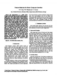
acoustic emission signal is amplified, goes though a high pass filter at 50KHz and feeds through a RMS meter with time constant of 8.0 ms. The vibration sensors are accelerometers with a frequency range up to 13KHz. They are also mounted to both table and spindle. The vibration signals are fed into a charge amplifier with sensitivity 5.71 and 100mV/g output, after which the signal is fed through a filter with corner frequencies 400Hz and 1KHz, and the RMS meter. The current converter powered by a triple output power supply providing 15V picks up the signal from one spindle motor current phase For data acquisition, a high speed data acquisition board (max. sampling rate of 100KHz) was used for all sensor inputs. We chose a 70mm face mill with 6 inserts using two types of inserts (Kennametal K420 and KC710) for roughing operations. Cutting speed was set to 200 m/min, depth of cut was 1.5mm and 0.75mm, feeds were 0.5m/rev and 0.25mm/rev, and two types of materials, cast iron and stainless steel J45, were used. Experiments for these 16 settings were run and then repeated to obtain independent training and test sets. ACOUSTIC EMISSION SENSOR SPINDLE

PREAMPLIFIER

RMS

ACOUSTIC EMISSION SENSOR TABLE

PREAMPLIFIER

RMS

VIBRATION SENSOR SPINDLE

CHARGE AMPLIFIER

LP/HP FILTER

RMS

VIBRATION SENSOR TABLE

CHARGE AMPLIFIER

LP/HP FILTER

RMS

COMPUTER

SPINDLE MOTOR CURRENT SENSOR

4. EXPERIMENTAL SETUP A milling machine under various operating environments was selected as the manufacturing environment. In particular, tool wear was investigated in a regular cut as well as entry and exit cuts. Data sampled by five different sensors, namely, two acoustic emission sensors (one on the table, one on the spindle), vibration sensors (one on the table, one on the spindle), and motor current sensor were used to determine the state of wear of the tool [33]. For wear measurement, flank wear VB (the distance from the cutting edge to the end of the abrasive wear on the flank face of the tool) was chosen. The flank wear was observed during the experiments by taking the insert out of the tool at roughly every 3 minutes and physically measuring the wear. The setup of the experiment is as depicted in Figure 1. The basic setup encompasses the spindle and the table of a Matsuura machine center MC-510V. An acoustic emission sensor with frequency range up to 2MHz is mounted to both the table and the spindle of the machine center. The

RECORDER

Fig. 1: Experimental Setup

5. FEATURE EXTRACTION The following features were extracted from each of the five sensor data resulting in a total of 25 features as listed in Table 1 a)

Windowed mean 1 u ( n) = x ( m) w( n − m) N where, N = window width w(n − m) = 1 when 0 ≤ n ≤ N − 1 = 0 otherwise

b) Windowed standard deviation

σ ( n) = c)

1 N

Kurtosis 1 κ ( n) = N

( x( m) − u ) 2 w(n − m)

( x(m) − u ) 4 w(n − m)

σ4

d) Short-time FFT with window-averaged magnitudes of the FFT spectra

SFFT ( k ) = DFT [ x ( m) w( n − m)]

=

x(m)w(n − m)e

−j

2π mk N

Table 1: Features DSP Raw

Sensors

Motor current Acoustic emission table Vibration table Acoustic emission spindle Vibration spindle Mean Motor current Acoustic emission table Vibration table Acoustic emission spindle Vibration spindle Stdev Motor current Acoustic emission table Vibration table Acoustic emission spindle Vibration spindle SFFT Motor current Acoustic emission table Vibration table Acoustic emission spindle Vibration spindle Kurtosis Motor current Acoustic emission table Vibration table Acoustic emission spindle Vibration spindle

Feature No. 1 2 3 4 5 6 7 8 9 10 11 12 13 14 15 16 17 18 19 20 21 22 23 24 25

6. RESULTS For the purpose of this examination, we chose data from one operating condition (cast iron, cutting speed: 200 m/min, depth of cut: 1.5mm, feed: 0.5m/rev) during steady state only. To first test our assumption, we performed training of the diagnostic model using the raw data alone and then the full set of features. In particular, a diagnostic neural network was trained with a 3-4-5 configuration, i.e., 3 input features, 4 nodes in a single hidden layer and 5 output nodes representing five wear classes. The neural net was trained for 1500 epochs with a learning rate of 0.1 and a momentum term of 0. 1. The training was repeated 10 times for each feature set to average the effect of random weight assignment. Mean test error and mean classification rate of the test set were taken as a performance measure to determine the best scheme. Using the raw data alone, the mean classification rate over the test set was 99.76% while the mean error of the test set was 1.4043. Using the full set of features, the mean classification error of the test set was 89.8% with a mean error of the test set of 5.4386. Both results do not give the desired performance, thus supporting our claim for need of feature selection. Table 2 summarizes the feature ranking based on each of the schemes. Table 2: Feature Ranking for top ten features Rank 1 2 3 4 5 6 7 8 9 10

Scatter Matrix 8 10 5 7 3 2 11 16 9 4

Cross Corr. 2 7 16 11 8 3 10 5 15 12

C4.5 2 3 5 7 8 10 11 16 15 9

ANFIS (par.) 8 10 11 16 15 2 24 9 7 5

ANFIS (sequ.) 11 8 7 5

To evaluate the five schemes, the three top ranked features were first selected from each scheme. Table 3 through Table 7 show the results of the 10 NN runs for the individual feature selection methods. With the exception of the crosscorrelation method, 100% classification rate and low test error can be achieved for all methods using three features. The distinction is mainly in the

average final test error which we take as a distinguishing means to rate performance of the feature selection tools. Here, sequential ANFIS yields slightly better results, followed by parallel ANFIS, the decision tree technique, the scatter matrix approach, and the cross-correlation approach. It must be noted that there is a chance that differences might be in part due to the randomized setup of the neural net weights which we tried to factor out to some degree by repeating the training process. In addition, overfitting problems and other effects may lead to a somewhat biased comparison. In terms of computational burden, the crosscorrelation method is the fastest, followed by the scatter matrix approach, C4.5, sequential ANFIS, and parallel ANFIS. However, we argue that the computational burden, even if it takes several hours (as in the case of parallel ANFIS) is not necessarily a big issue in the design of a diagnostic system which may last several months. Besides the synergistic value of features sets, another inherent danger in sequential feature selection is that partially redundant features are chosen repeatedly. Choosing similar features is correct for the individual decision at the time but not from the vantage point of overall performance. Therefore, features that have a higher degree of independence are to be preferred in the selection process. Here, approaches that select several features at a time, such as both ANFIS approaches, have a tremendous advantage. This may explain why the approaches using the sequential strategies rate slightly behind the strategies using the simultaneous evaluation. In case of the scatter matrix approach, for example, features 10 and 5 have a higher degree of redundancy than the top features chosen by ANFIS.

Mean error of test set: 0.38198; mean classification rate of test set: 100% Table 4: NN Training for cross-correlation features Train error

Classificat Test Classification error rate ion rate (train set) (test set) 3.5789 94.8 8.1639 82.8 4.4866 94 3.4245 96.4 4.7413 93.2 3.0462 97.6 3.4791 95.6 8.2807 82.4 4.3201 93.2 8.0414 82.8 4.2833 94.4 3.7066 95.6 4.1344 94.4 3.9943 94.8 3.5253 95.2 8.3714 82.4 3.5248 95.2 8.2623 82.4 3.7828 96 4.7365 92.4 Mean error test set: 6.0028; mean classification rate test set: 88.96%

Table 5: NN Training for C4.5 features Train error

Classificat Test Classification ion rate error rate (test set) (train set) 0.29611 100 0.35246 100 0.34154 100 0.41306 100 0.32204 100 0.47199 100 0.30364 100 0.46659 100 0.24825 100 0.29985 100 0.31905 100 0.49921 100 0.2606 100 0.30756 100 0.26663 100 0.31296 100 0.27771 100 0.30741 100 0.27174 100 0.3184 100 Mean error of test set: 0.37495; mean classification rate of test set: 100%

Table 3: NN Training for scatter matrix features Train error 0.3704 0.36206 0.35395 0.26327 0.34358 0.37333 0.35057 0.26115 0.34355 0.3491

Class. rate (train set) 100 100 100 100 100 100 100 100 100 100

Test error 0.38558 0.38381 0.41485 0.30763 0.42389 0.39774 0.41224 0.28804 0.41983 0.38618

Class. rate (test set) 100 100 100 100 100 100 100 100 100 100

Table 6: NN Training for parallel ANFIS features Train error 0.34915 0.32448 0.31726 0.34302 0.35666 0.31309 0.37059 0.3234 0.36405

Class. rate (train set) 100 100 100 100 100 100 100 100 100

Test error 0.30317 0.34123 0.25512 0.2865 0.30858 0.39802 0.31855 0.26573 0.31997

Class. rate (test set) 100 100 100 100 100 100 100 100 100

0.30039 100 0.273 100 Mean error test set: 0.30699; mean classification rate test set: 100%

Table 7: NN Training for sequential ANFIS features Train Class. rate Test error Class. rate error (train set) (test set) 0.28539 100 0.33498 100 0.27568 100 0.25788 100 0.25825 100 0.24282 100 0.28407 100 0.26313 100 0.295 100 0.27268 100 0.2951 100 0.28584 100 0.27007 100 0.27457 100 0.29246 100 0.28147 100 0.27515 100 0.26068 100 0.27024 100 0.25125 100 Mean error of test set: 0.27253; mean classification rate of test set: 100%

7. CONCLUSIONS All five selection schemes considered in this paper can rank the features without going through optimal search (although the simultaneous evaluation of ANFIS is an exhaustive enumeration). Given the sensor data from the experiment for milling tool wear, the complementary approaches using ANFIS outperformed the sequential approaches. By carefully examining the results from all of the selection schemes, we can see that in this case features extracted by windowed mean process tend to have more classification power than other processes, particularly, the windowed means of vibration signals. Features extracted from kurtosis process tend to fall into the less important group. However, one should not generalize from these findings to the quality of these features in general which have been established to be powerful in other instances. Since we selected one operating condition at steady state from the set of data, the classification rates are fairly high for all feature selection methods. While we plan to expand the experiments presented here to encompass all operating conditions, we anticipate that the feature selection results can be qualitatively extrapolated from the ones presented here.

Future work should consider using information fusion to combining the results from different selection schemes for more complex and ambiguous feature selection scenarios. This work here does not claim to have an exhaustive set of features. Rather, applying more DSP techniques, such as, wavelet transform, CEPSTRUM, etc. to the raw sensor signals to extract more features should also be considered, in particular when considering the full set of data. Finally, we only partially addressed the issue of optimal number of features. The approach chosen here can be extended to select the minimum number of features in an efficient manner by sequentially increasing the number of features starting from one.

Acknowledgements We thank Profs. Agogino, Dornfeld, and Tomizuka (all of UC Berkeley) and Drs. Dvorak and Sokolowski for helping with the experiments. We also thank Drs. Chen and Bonissone for helpful discussions and suggestions on this subject

References [1] K. Kira and L. Rendell, “The Feature Selection Problem: Tranditional Methods and a New Algorithm”, AAAI-92, pp129-134, 1992. [2] M., Dash, H. Liu, “Feature Selection for Classification”, Intelligent Data Analysis, Vol.1, No.3, August, 1997. [3] H. Liu, H. Motoda, “ Feature Selection for Knowledge Discovery and Data Mining”, Kluwer Academic Publishers, Norwell, MA,1998. [4] P. Narendra, K. Fukunaga, “A Branch and Bound Algorithm for Feature Subset Selection”, IEEE Transactions on Computer, Vol.C-26, No.9, pp917-922, 1977. [5] J. Kitter, “Feature Set Search Algorithm’, Pattern Recognition and Signal Processing, Sithoff and Noordhoff, Alphen ann Den Riju, The Netherlands, pp41-60, 1978. [6] P. Pudil, J. Novovicova, J. Kittler, “ Floating Search Methods in Feature Selection”, Pattern Recognition Letters 15 (1), pp1119-1125, 1994. [7] C. Cardie, “Using Decision Trees to Improve Case-Based Learning”, Proceedings of 10th International Conference on Machine Learning, pp25-32, 1993. [8] J. Yang and V. Honavar, “Feature Subset Selection Using a Genetic Algorithm”, IEEE Intelligent Systems, Vol. 13, No.2, pp44-49, 1998. [9] J. Doak, “An Evaluation of Feature Selection Methods and their Application to Computer

Security”, Technical report, Davis, CA: University of California, Department of Computer Science, 1992. [10] I. Inza, et cl, “Feature Subset Selection By Bayesian Networks Based Optimization”, Technical Report, EHU-KZAA-IK-2/99, University of the Basque Country. http://www.sc.ehu.es/ccwbayes/publics.htm [11] S. Pal, “Fuzzy Set Theoretic Measures for Automatic Feature Evaluatio:II”, Information Science, Vol.64, pp165-179, 1992. [12] M. Ramze Rezaee, B. Goedhart, B. Lelieveldt, “Fuzzy Feature Selection”, Patern Recognition, Vol. 32, No.12, pp2011-2019, 1999. [13] S. Pal, J. Basak, R. De, “Feature Selection: a Neuro-fuzzy Approach”, ICNN96, The 1996 IEEE International Conference on Neural Networks”, Vol.2, pp1197-1202, 1996. [14] R. Setiono, H. Liu, “Neural-Network Feature Selector”, IEEE Transactions on Neural Networks, Vol. 8, No. 3, pp 654-662, 1997. [15] N. Kasabov, et cl, “Neural Networks for Feature Selection”, Proceedings of the 1997 International Conference on Neural Information Processing and Intelligent Information Systems, Vol.2, pp1121-1124, 1998. [16] R. Duda and P. Hart, “Pattern Classification and Scene Analysis”, Wiley, New York, 1973. [17] S. Piramuthu, “The Hausdorff Distance Measure for Feature Selection in Learning Applications”, Proceedings of the 32nd Annual Hawaii International Conference on Systems Sciences, 1999. [18] T. Chan, “A Fast Metric Approach to Feature Subset Selection”, Proceedings of 24th EUROMIRO Conference, Vol. 2, pp733-736, 1998. [19] H. Almuallim, T. Dietterich, “Learning Boolean Concepts in Presence of Many Irrelevant Features”, Artificial Intelligence, pp279305,November,1994. [20] M. Ben-Bassat, “Pattern Recognition and Reduction of dimensionality”, Handbook of Statistics (P. Krishnaiah and L. Kanal, eds.) North Holland, pp773-791, 1982. [21] M. Hall, L. Smith, “Feature Subset Selection: a Correlation Based Filter Approach”, Proceedings of the 1997 International Conference on Neural Information Processing and Intelligent Information Systems, Vol. 2, pp855-858, 1998 [22] G. John, R. Kohavi, and K. Pfleger, “Irrelevant Features and the Subset Selection Problems”, Proceedings of 11th Int’l Conference on Machine Learning, San Mateo, CA, pp121-129, 1994. [23] H. Wang, D. Bell, and F. Murtagh, “Axiomatic Approach to Feature Subset Selection Based on Relevance”, IEEE Transactions on Pattern Analysis

and Machine Intelligence, Vol. 21, No.3, pp271277, 1999. [24] P. Langley, “Selection of Relevant Features in Machine Learning”, Proceedings of 1994 AAAI Fall Symposium, pp127-131, 1994. [25] M. Boussouf, “A Hybrid Approach to Feature Selection”, Proceedings of Principles of Data Mining and Knowledge Discovery, 2nd European Symposium, PKDD’98, pp230-238, 1999. [26] A.J. Miller, “Subset Selection in Regress”, Chapman and Hall, Washington DC, 1990. [27] S. Stearns, “On Selecting Features for Pattern Classifiers”, Proceedings of the 3rd International Conference on Pattern Recognition, Coronado, CA 1976, pp71-75. [28] A. Blum, and P. Lanfley, “Selection of Relevant Features and Examples in Machine Learning”, Artificial Intelligence 97, pp245-271, 1997. [29] M. Chen, J. Han, and P. Yu, “Data Mining: An Overview from Database Perspective”, IEEE Transactions on Knowledge and Data Engineering, Vol. 8, No. 6, pp866-883, 1996. [30] W. Graco, R. Cooksey, “Feature Selection with Data Mining”, FADD98, Proceedings of 2nd International Conference on the Practical Application of Knowledge Discovery and Data Mining, pp111-130, 1998. [31] L. Jack, A. Nandi, “ Feature Selection for ANNs Using Genetic Algorithms in Condition Monitoring”, Proceedings of 7th European Symposium on Artificial Neural Networks, ESANN’99, pp313-318, 1999. [32] F. Pan, A. Hope, G. King, “A Neuro-fuzzy Classification Network and its Application”, Proceedings of 1998 IEEE International Conference on Systems, Man, and Cybernetics, Vol. 5, pp42344239, 1999. [33] K. Goebel, “Using a Neural-Fuzzy Scheme to Diagnose Manufacturing Processes”, Master’s thesis, UC Berkeley, 1993. [34] J. Quinlan, “C4.5: Programs for Machine Learning”, Morgan Kaufmann, San Mateo, CA, 1993. [35] J.-S. R. Jang, “Input Selection for ANFIS Learning”, Proceedings of the Fifth IEE International Conference on Fuzzy Systems FUZZIEEE ‘96, pp1493-1499,1996. [36] J.-S. R. Jang, C.-T. Sun, and E. Mizutani, “Neuro-Fuzzy and Soft Computing”, Prentice Hall, Upper Saddle River, NJ, 1997. [37] J. Li, “Mechanical Diagnostics”, Lecture Notes, 1999.