FIFTH AND SIXTH-ORDER ITERATIVE ALGORITHMS WITHOUT ...

International Journal of Pure and Applied Mathematics Volume 83 No. 1 2013, 111-119 ISSN: 1311-8080 (printed version); ISSN: 1314-3395 (on-line version) url: http://www.ijpam.eu doi: http://dx.doi.org/10.12732/ijpam.v83i1.10

AP ijpam.eu

FIFTH AND SIXTH-ORDER ITERATIVE ALGORITHMS WITHOUT DERIVATIVES FOR SOLVING NON-LINEAR EQUATIONS G. Fern´ andez-Torres1 § , F.R. Castillo-Soria2 , I. Algredo-Badillo3 1 Petroleum

Engineering Department Universidad del Istmo ´ Tehuantepec, Oaxaca, 70760, MEXICO 2 Computer Engineering Department Universidad del Istmo ´ Tehuantepec, Oaxaca, 70760, MEXICO

Abstract: In this paper we will present two derivative free iterative methods for finding the root of a nonlinear equation f (x) = 0. The new methods are based on direct and inverse polynomial interpolation. We will prove that one of the methods has fifth-order convergence and the other method sixth-order convergence. Several examples will show that convergence and the efficiency of the new methods to be better than the classic Newton’s method and others derivative free methods with high order of convergence previously presented. AMS Subject Classification: 65D05, 65D07, 65D15 Key Words: nonlinear equations, iterative methods, roots finding method, derivative free, interpolation

1. Introduction There are several different methods in the literature to compute the root r of a Received:

November 15, 2012

§ Correspondence

author

c 2013 Academic Publications, Ltd.

url: www.acadpubl.eu

112

G. Fern´ andez-Torres, F.R. Castillo-Soria, I. Algredo-Badillo

nonlinear equation f (x) = 0. The most famous of these methods is the classical Newton’s method f (xn ) xn+1 = xn − ′ , (1) f (xn ) starting from some initial value x0 with convergence order 2. If the derivative f ′ (xn ) is replaced by the forward difference approximation f ′ (xn ) ≈

f (xn + f (xn )) − f (xn ) f (xn )

(2)

we obtain the classical Steffensen’s method xn+1 = xn −

f 2 (xn ) . f (xn + f (xn )) − f (xn )

(3)

Both the above methods have an order of convergence 2 and require two functional evaluations per iteration. However Steffensen’s method is free from any derivative of the function. This is important because sometimes, in science and engineering, the applications of the iterative methods which depend upon derivatives are restricted. In recent years several researchers have developed iterative methods for solving nonlinear equations. These methods have been developed using error analysis techniques, quadrature rules and other techniques, see [2, 6, 8, 13]. Most recently, a derivative free Steffensen-secant method was proposed by Jain [4]. It uses three functional evaluations per step and has cubic convergence. In [14] a family of Steffensen like methods was derived by Zheng by applying forward difference approximation to the Weerakoon and Fernando method [13], which has cubic convergence and uses four functional evaluations per iteration. In a similar way Cordero [3] used central difference approximation f ′ (xn ) ≈

f (xn + f (xn )) − f (xn − f (xn )) 2f (xn )

(4)

in the Ostrowski’s fourth-order method [9], obtaining a new method. This new method, free from derivatives, has fourth order convergence and requires four functional evaluations per iteration.

2. Develop of the Methods Consider a function sufficiently differentiable f (x) with f ′ (x) 6= 0 on an open interval I and r ∈ I a simple zero of f (x). Since r and f ′ (x) 6= 0 is a simple

FIFTH AND SIXTH-ORDER ITERATIVE ALGORITHMS...

113

zero we can consider g = f −1 on I. Suppose that the process starting with x0 ∈ I close to r and xn has been chosen. Define t1 = xn + f (xn ), t2 = xn − f (xn ),

(5)

L0 = f (xn ), L1 = f (t1 ), L2 = f (t2 ).

(6)

Using the notation of divided differences, consider the following interpolating polynomial for f (x) p(x) = A(x − xn )(x − t1 ) + B(x − xn ) + C

(7)

A = f [xn , t1 , t2 ], B = f [xn , t1 ], C = f [xn ],

(8)

where and verify p(xn ) = L0 , p(t1 ) = L1 , p(t2 ) = L2 . Solving the polynomial p1 (x) = [−AL0 + B](x − xn ) + C = 0

(9)

we obtain the following two-step derivative free method (FCAM1) as follows y n = xn − xn+1

=

f [xn ] , L3 = f (yn ) f [xn , t1 ] − f [xn , t1 , t2 ]f (xn ) 3 X (−1)i g[L0 , . . . , Li ]L0 · · · Li−1 . xn +

(10) (11)

i=1

Now, consider the following interpolating polynomial for g(y) s(y) = A(y − L0 )(y − L1 ) + B(y − L0 ) + C

(12)

A = g[L0 , L1 , L2 ], B = g[L0 , L1 ], C = g[L0 ],

(13)

where with s(L0 ) = g(L0 ) = xn , s(L1 ) = g(L1 ) = t1 , s(L2 ) = g(L2 ) = t2 . Defining yn = s(0) we obtain the following new two-step derivative free method (FCAM2) as follows yn

2 X (−1)i g[L0 , . . . , Li ]L0 · · · Li−1 , L3 = f (yn ), = xn +

(14)

i=1

xn+1 = yn − g[L0 , . . . , L3 ]L0 · · · L2 .

(15)

114


Observe that in (11) and (15) we have used inverse interpolation on the points Li , for 1 ≤ i ≤ 3, with the polynomial q(y) = g[L0 ] +

3 X

g[L0 , . . . , Li ](y − L0 ) · · · (y − Li−1 ).

(16)

i=1

The computational efficiency of an iterative method of order p, requiring N function evaluations per iteration, is most frequently calculated by OstrowskiTraub’s efficiency index [9, 12] 1

E = pN .

(17)

It can be seen that the methods (FCAM1), (FCAM2) require four function 1 1 evaluations per iteration with efficiency indexes (5) 4 ∼ 1.495 and (6) 4 ∼ 1.565, respectively. These efficiency indexes are clearly superior to the efficiency indexes of Steffensen’s and Newton’s methods which are equal to 1.414.

3. Order of Convergence Theorem 1. Let f : I ⊆ R → R be a sufficiently differentiable function and let r ∈ I be a simple zero of f (x) = 0 in an open interval I, with f (x) 6= 0 on I. Define g = f −1 on I. If x0 ∈ I is sufficiently close to r, then the method free from derivatives (FCAM1) defined by (10) and (11) has order of convergence 5. Proof. First, from (7) and (9) we have p(x) = A(x − xn )2 + p1 (x) then, the error for the polynomial p1 (x) can be written as f (x) − p1 (x) =

f ′′′ (ξ2 ) f ′′ (ξ1 ) (x − xn )2 + (x − xn )(x − t1 )(x − t2 ), 2 6

(18)

for some ξ1 , ξ2 ∈ I. Substituting t1 , t2 , evaluating in x = r and taking ǫn = xn − r we have p1 (r) = −

f ′′ (ξ1 ) 2 f ′′′ (ξ2 ) ǫn + ǫn (ǫn + f (xn ))(ǫn − f (xn )). 2 6

(19)

Note that if we expand f (xn ) with Taylor’s polynomial of first degree around r, the second term in the right side can be written, for some ξ3 ∈ I, as f ′′′ (ξ2 ) 3 f ′′′ (ξ2 ) ǫn (ǫ2n − f 2 (xn )) = ǫn (1 − (f ′ (ξ3 ))2 ) = O(ǫ3n ). 6 6

(20)


115

′′

1) ′ ′ Now, since p′1 = −AL0 + B = − f (ξ 2 f (ξ3 )ǫn + f (ξ4 ), for some ξ4 ∈ I, expanding p1 (r) around yn with ǫn+1 = r − yn , we have, from (19), the following asymptotic equation

yn − r ∼ −

f ′′ (ξ1 ) 2 ǫ + O(ǫ3n ). 2f ′ (ξ4 ) n

(21)

In the same way, the error for the polynomial q(y) given by (16) is g(y) − q(y) =

g(4) (η) (y − L0 )(y − L1 )(y − L2 )(y − L3 ), 24

(22)

for some η ∈ f (I). Expanding, f (xn + f (xn ), f (xn − f (xn )) and f (yn ) with Taylor’s polynomial of first degree around r, we have, for some ξ5 , ξ6 , ξ7 ∈ I, f (xn + f (xn )) = f ′ (ξ5 )(xn − r + (xn − r)f ′ (ξ3 )), ′

′

f (xn − f (xn )) = f (ξ6 )(xn − r − (xn − r)f (ξ3 )), ′

f (yn ) = (yn − r)f (ξ7 ).

(23) (24) (25)

Thus, substituting y = 0 in (22) with ǫn+1 = xn+1 − r, and using (21) we have the following asymtotic equation ǫn+1 ∼ −

f ′′ (ξ1 ) g(4) (η) 5 ′ ǫn f (ξ3 )f ′ (ξ5 )f ′ (ξ6 )f ′ (ξ7 )(1 − (f (ξ3 ))2 ) ′ + O(ǫ6n ), (26) 24 2f (ξ4 )

and finally ǫn+1 ∼ kǫ5n

(27)

with k as a suitable constant. Theorem 2. Let f : I ⊆ R → R be a sufficiently differentiable function and let r ∈ I be a simple zero of f (x) = 0 in an open interval I, with f (x) 6= 0 on I. Define g = f −1 on I. If x0 ∈ I is sufficiently close to r, then the method free from derivatives (FCAM2) defined by (14) and (15) has an order of convergence of 6. Proof. First, from (12) the error for the polynomial s(y) can be written as g(y) − s(y) =

g′′′ (η1 ) (y − L0 )(y − L1 )(y − L2 ). 6

(28)

Evaluating in y = 0, and expanding L0 , L1 , L2 as in (23), (24) and (25) we obtain g′′′ (η1 ) 3 ′ ǫn f (ξ3 )f ′ (ξ5 )f ′ (ξ6 )(1 − (f (ξ3 ))2 ). (29) yn − r = 6

116


Now, for the polynomial in (16) the error can be written as g(y) − q(y) =

g′′′ (η2 ) (y − L0 )(y − L1 )(y − L2 )(y − L3 ). 6

(30)

Evaluating in y = 0, and expanding L0 , L1 , L2 , L3 as before we obtain ǫn+1 = −

gIV (η1 ) 6 ′2 ǫn f (ξ3 )f ′2 (ξ5 )f ′2 (ξ6 )(1 − (f (ξ3 ))2 )2 . 6

(31)

and finally ǫn+1 ∼ kǫ6n

(32)

with k as a suitable constant.

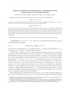
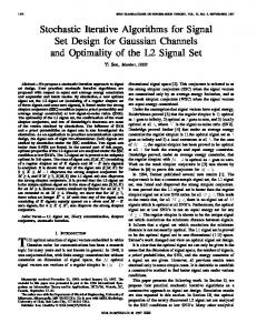
4. Numerical Examples In this section we use numerical examples to compare the methods introduced in this paper. (FCAM1) and (FCAM2) are compared with methods that do not use derivatives such as Steffensens (SM), Cordero’s (CM), Jain’s (JM) [4] and Zheng’s methods (ZM) [14]. We also compare methods that use derivatives such as Newton’s (NM), Chun’s (CHM) [2], Kou’s (KM) [5] and Noor’s methods (NOM) [7]. All computations were carried out with double arithmetic precision on MATLAB 10. Table 1 and Table 2 show the number of iterations and the number of functional evaluations required such that |f (xn )| < 10−17 . Numerical results show that the new derivative free methods (FCAM1) and (FCAM2) can compete with Newton’s method and Steffensens method and converge faster than (JM) and (ZM), in many cases. We use the following functions, some of which are the same as in the derivative free methods [2, 3, 4, 5, 6, 7, 8, 13, 14] respectively. Modern applications have high computational requirements in a many variety of fields, including financial analysis, data mining, medical imaging, and scientific computation. In many applications, implementations on FPGA report better results and computation times than software implementation methods, such as Newton-Rapshon, Non-Restoring Square Root [10], Bisection, Lanczos [11] and secant Volterra methods [1], among others. Future work will be needed to implement the proposed methods on high-performance FPGA-based systems for obtaining implementation results.

FIFTH AND SIXTH-ORDER ITERATIVE ALGORITHMS... f1 (x) = cos(x) − x, f2 (x) = (x − 1)3 − 2, f3 (x) = (x − 1)2 − 1, f4 (x) = x3 + 4x2 − 10, f5 (x) = sin(x) − 12 x, f6 (x) = sin2 (x) − x2 + 1, f7 (x) = x2 − ex − 3x + 2, 2 f8 (x) = xex − sin2 (x) + 3 cos(x) + 5,

f (x)

f1 (x) f2 (x) f3 (x) f4 (x) f5 (x) f6 (x) f7 (x) f8 (x)

r = 0.7390851332151606. r = 2.2599210498948731. r = 2. r = 1.3652300134140968. r = 1.8954942670339809. r = 1.4044916482153412. r = 0.2575302854398607. r = 1.2076478271309189.

Iterations - NFE

x0

0.5 1.85 3.5 1 2 1.5 3 -3

117

SM 4-8 6 - 12 6 - 12 5 - 10 4-8 4-8 6 - 12 14 - 28

JM 3-9 6 - 18 4 - 12 4 - 16 3 - 12 3 - 12 4 - 16 10 - 40

ZM 3 - 12 6 - 24 4 - 16 4 - 12 3-9 3-9 4 - 12 10 - 30

CM 2-8 4 - 16 3 - 12 3 - 12 2-8 2-8 3 - 12 8 - 32

FCAM1

FCAM2

2-8 3 - 12 3 - 12 3 - 12 2-8 2-8 3 - 12 7 - 28

2-8 3 - 12 3 - 12 2-8 2-8 2-8 3 - 12 6 - 24

Table 1: Comparison with derivative free methods

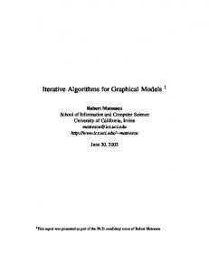
5. Conclusions The problem of locating roots of nonlinear equations (or zeros of functions) occurs frequently in scientific work. In this paper, we have introduced two new techniques for solving nonlinear equations. The introduced methods can be used for solving nonlinear equations without computing derivatives. We have proven that one method has fifth-order convergence and the other has sixthorder convergence. The efficiency indexes of the methods are 1.495 and 1.565 greater than the efficiency index of Newton’s and Steffensen’s methods. The numerical examples show the greater efficiency of the new methods, especially (FCAM2).

118


f (x)

f2 (x) f4 (x) f6 (x) f7 (x) f8 (x)

Iterations - NFE

x0

3 1 1 2 0 1 -2

NM 7 - 14 6 - 12 7 - 14 6 - 12 5 - 10 5 - 10 9 - 18

CHM 4 - 12 4 - 12 4 - 12 4 - 12 4 - 12 4 - 12 5 - 15

KM 6 - 24 4 - 12 5 - 15 4 - 12 3-9 3-9 6 - 18

NOM 4 - 16 3 - 12 3 - 12 3 - 12 3 - 12 3 - 12 4 - 16

FCAM1 3 - 12 3 - 12 4 - 16 3 - 12 2-8 3 - 12 5 - 20

FCAM2 3 - 12 2-8 3 - 12 3 - 12 2-8 2-8 4 - 16

Table 2: Comparison with methods that use derivatives Acknowledgments The authors wish to acknowledge the valuable participation of Professors Ted Fondulas and Alex Yealland in the proof-reading of this paper. The third author has been financially supported by PROMEP (UNISTMONPTC-056 Ignacio Algredo Badillo).

References [1]

E. Aschbacher et. al., Prototype implementation of two efficient lowcomplexity digital predistortion algorithms, EURASIP Journal on Advances in Signal Processing, Vol. 2008 (2008).

[2]

C. Chun, A family of composite fourth-order iterative methods for solving nonlinear equations, Applied Mathematics and Computation, 187 (2007), 951-956.

[3]

A. Cordero et. al., Steffensen type methods for solving nonlinear equations, Journal of Computational and Applied Mathematics, 236 (2012), 30583064.

[4]

P. Jain, Steffensen type methods for solving nonlinear equations, Applied Mathematics and Computation, 194 (2007), 527-533.


119

[5]

J. Kou, Y. Li and X. Wang, A composite fourth-order iterative method for solving non-linear equations, Applied Mathematics and Computation, 184 (2007), 471-475.

[6]

J. Kou, Y. Li and X. Wang, A modification of Newton method with thirdorder convergence, Applied Mathematics and Computation, 181 (2006), 1106-1111.

[7]

M. A. Noor, W. A. Khan and A. Hussain, A new modified Halley method without second derivatives for nonlinear equation, Applied Mathematics and Computation, 189 (2007), 1268-1273.

[8]

K. I. Noor, M. A. Noor, Predictor-corrector Halley method for nonlinear equations, Applied Mathematics and Computation, 188 (2007), 1587-1591.

[9]

A. M. Ostrowski, Solution of equations and systems of equations, Academic Press, New York (1960).

[10] K. Piromsopa, C. Aporntewan, P. Chongsatitvatana, An FPGA implementation of a fixed-point square root operation, 2001 International Symposium on Communications and Information Technology (ISCIT’2001), Thailand (2001). [11] A. Rafique, N. Kapre, and G. A. Constantinides, A high throughput FPGA-based implementation of the Lanczos method for the symmetric extremal eigenvalue problem, ARC (2012), 239-250. [12] J. F. Traub, Iterative Methods for the Solution of Equations, Prentice Hall, New York (1964). [13] S. Weerakoon, T.G.I. Fernando, A variant of Newton’s method with accelerated third-order convergence, Applied Mathematics Letters, 13 (2000), 87-93. [14] S. Zheng et. al., A Steffensen-like method and its higher-order variants, Applied Mathematics and Computation, 214 (2009), 10-16.

120