Finding Meter in Music Using an Autocorrelation Phase Matrix and Shannon Entropy Douglas Eck University of Montreal Department of Computer Science CP 6128, Succ. Centre-Ville Montreal, Quebec H3C 3J7 CANADA
[email protected]
ABSTRACT This paper introduces a novel way to detect metrical structure in music. We introduce a way to compute autocorrelation such that the distribution of energy in phase space is preserved in a matrix. The resulting autocorrelation phase matrix is useful for several tasks involving metrical structure. First we can use the matrix to enhance standard autocorrelation by calculating the Shannon entropy at each lag. This approach yields improved results for autocorrelationbased tempo induction. Second, we can efficiently search the matrix for combinations of lags that suggest particular metrical hierarchies. This approach yields a good model for predicting the meter of a piece of music. Finally we can use the phase information in the matrix to align a candidate meter with music, making it possible to perform beat induction with an autocorrelation-based model. We present results for several meter prediction and tempo induction datasets, demonstrating that the approach is competitive with models designed specifically for these tasks. We also present preliminary beat induction results on a small set of artificial patterns. Keywords: Meter prediction, tempo induction, beat induction, autocorrelation, entropy
1 Introduction In this paper we introduce an autocorrelation phase matrix, a two-dimensional structure (computed from MIDI or digital audio) that provides the necessary information for estimating the lags and phases of the music’s metrical hierarchy. We use this matrix as the core data structure to estimate the meter of a piece (meter prediction), to estimate the tempo of a piece (tempo induction) and to align the piece of music with the predicted metrical structure (beat induction). We will provide algorithm details and experimental rePermission to make digital or hard copies of all or part of this work for personal or classroom use is granted without fee provided that copies are not made or distributed for profit or commercial advantage and that copies bear this notice and the full citation on the first page. c
2005 Queen Mary, University of London
504
Norman Casagrande University of Montreal Department of Computer Science CP 6128, Succ. Centre-Ville Montreal, Quebec H3C 3J7 CANADA
[email protected]
sults for meter prediction and tempo induction. We will also present some details concerning the alignment of the metrical structure with a piece of music. We will also present alignment results for a small dataset of artificial patterns. However the details of computing this alignment online (for beat induction) are the topic of another paper. The structure of this paper is as follows. In Section 2 we will discuss other approaches to finding meter and beat in music. In Section 3 we will describe our model consisting of the creation of an autocorrelation matrix, computation of the entropy for each lag in this matrix, the selection of a metrical hierarchy and the alignment of the hierarchy with music. Finally in Section 4 we present simulation results. Due to space constraints we have omitted details for aligning the autocorrelation phase matrix with a musical signal so as to aid in beat induction. A longer report containing these details is available at www.iro.umontreal.ca/˜eckdoug/ publications.html.
2
Meter and Autocorrelation
Meter is the sense of strong and weak beats that arises from the interaction among hierarchical levels of sequences having nested periodic components. Such a hierarchy is implied in Western music notation, where different levels are indicated by kinds of notes (whole notes, half notes, quarter notes, etc.) and where bars establish measures of an equal number of beats (Handel, 1993). For instance, most contemporary pop songs are built on fourbeat meters. In such songs, the first and third beats are usually emphasized. Knowing the meter of a piece of music helps in predicting other components of musical structure such as the location of chord changes and repetition boundaries (Cooper and Meyer, 1960). Autocorrelation works by transforming a signal from the time domain into the frequency domain. Autocorrelation provides a high-resolution picture of the relative salience of different periodicities, thus motivating its use in tempo and meter related music tasks. However, the autocorrelation transform discards all phase information, making it impossible to align salient periodicities with the music. Thus autocorrelation can be used to predict, for example, that music has something that repeats every 1000ms but it cannot say when the repetition takes place
3 3.1
Model Details
Preprocessing
For MIDI files, the onsets can be transformed into spikes with amplitude proportional to their midi note onset volume. Alternately MIDI files can simply be rendered as audio and written to wave files. Stereo audio files are converted to mono by taking the mean of the two channels. Then files are downsampled to some rate near 1000Hz. The actual rate is kept variable because it depends on the original sampling rate. For CD-audio (44.1Khz), we used a sampling rate of 1050Hz allowing us to downsample by a factor of 42 from the original file. Best results were achieved by computing a sum-of-squares envelope over windows of size 42 with 5 points of overlap. However for most audio sources a simple decimation and rectification works as well. The model was not very sensitive to changes in sampling rate nor to minor adjustments in the envelope computation such as substituting RMS (root mean square) for the sum of squares computation. 3.2
Autocorrelation Phase Matrix
Autocorrelation is a special case of cross-correlation where x1 == x2 . There is a strong and somewhat surprising link between autocorrelation and the Fourier trans-
form. Namely the autocorrelation A of a signal X (having length N ) is: A(X)
=
(1)
if f t(|f f t(X)|)
where f f t is the (fast) Fourier transform, if f t is the inverse (fast) Fourier transform and || is the complex modulus. One advantage of autocorrelation for our purposes is that it is defined over periods rather than frequencies (note the application of the IFFT in Equation 1), yielding better representation of low-frequency information than is possible with the FFT. Autocorrelation values for a random signal should be roughly equal across lags. Spikes in an autocorrelation indicate temporal order in a signal, making it possible to use autocorrelation to find the periods at which high correlation exists in a signal. As a music example, consider the autocorrelation for a ChaChaCha from the ISMIR 2004 Tempo Induction contest is shown (Figure 1). The peaks of the autocorrelation align with the tempo and integer multiples of the tempo.
autocorrelation
Albums−Cafe_Paradiso−08.wav 400 350 300
Target tempo = 483.9 ms (124.0 BPM) 0
500
1000
1500
2000 lag (msec)
2500
3000
3500
4000
Figure 1: Autocorrelation of a ChaChaCha from the ISMIR 2004 Tempo Induction contest (Albums-Cafe Paradiso-08.wav). The dotted vertical lines mark the actual tempo of the song (484 msec, 124 bpm) and harmonics of the tempo. Unfortunately autocorrelation has been shown in practice to not work well for many kinds of music. For example when a signal lacks strong onset energy, as it might for voice or smoothly changing musical instruments like strings, the autocorrelation tends to be flat. See for example a song from Manos Xatzidakis from the ISMIR 2004 Tempo Induction in Figure 2. Here the peaks are less sharp and are not well-aligned with the target tempo. Note that the y-axis scale of this graph is identical to that in Figure 1. 15−AudioTrack 15.wav autocorrelation
relative to the start of the music. One primary goal of our work here is to compute autocorrelation efficiently while at the same time preserving the phase information necessary to perform such an alignment. Our solution is the autocorrelation phase matrix. Autocorrelation is certainly not the only way to perform meter prediction and related tasks like tempo induction. Adaptive oscillator models (Large and Kolen, 1994; Eck, 2002) can be thought of as a time-domain correlate to autocorrelation based methods and have shown promise, especially in cognitive modeling. Multi-agent systems such as those by Dixon (2001) have been applied with success. as have Monte-Carlo sampling (Cemgil and Kappen, 2003) and Kalman filtering methods (Cemgil et al., 2001). Many researchers have used autocorrelation for music information retrieval. Due to space constraints only a short listing is provided here. Brown (1993) used autocorrelation to find meter in musical scores represented as note onsets weighted by their duration. Vos et al. (1994) proposed a similar autocorrelation method. The primary difference between their work and that of Brown was their use of melodic intervals in computing accents. Scheirer (1998) provided a model of beat tracking that treats audio files directly and performs relatively well over a wide range of musical styles (41 correct of 60 examples). Volk (2004) explored the influence of interactions between levels in the metrical hierarchy on metrical accenting. Toiviainen and Eerola (2004) also investigated an autocorrelation-based meter induction model. Their focus was on the relative usefulness of durational accent and melodic accent in predicting meter. Klapuri et al. (2005) incorporate the signal processing approaches of Goto (2001) and Scheierer in a model that analyzes the period and phase of three levels of the metrical hierarchy.
500 480 Target tempo = 563.0 ms (106.6 BPM)
460 0
500
1000
1500
2000 lag (msec)
2500
3000
3500
4000
Figure 2: Autocorrelation of a song by Manos Xatzidakis from the ISMIR 2004 Tempo Induction contest (15-AudioTrack 15.wav). The dotted vertical lines mark the actual tempo of the song (563 msec, 106.6 bpm) and harmonics of the tempo. One way to address this is to apply the autocorrelation to a number of band-pass filtered versions of the signal, as discussed in Section 3.1. In place of multi-band processing we compute the distribution of autocorrelation energy in phase space. This has a sharpening effect, allowing autocorrelation to be applied to a wider range of signals than autocorrelation alone without extensive preprocessing.
505
The autocorrelation phase information for lag l is a vector Al :
b N l−l c
Al =
X i=0
l−1
xli+φ xl(i+1)+φ
(2)
φ=0
We compute an autocorrelation phase vector Al for each lag of interest. In our case the minimum lag of interest was 200ms and the maximum lag of interest was 3999ms. Lags were sampled at 1ms intervals yielding L = 3800 lags. Equation 2 effectively “wraps” the signal modulo the lag l question, yielding vectors of differing lengths (|Al | == l). To simplify later computations we normalized the length of all vectors by resampling. This was achieved by fixing the number of phase points for all lags at K (K = 50 for all simulations; larger values were tried and yielded similar results but significantly smaller values resulted in a loss of temporal resolution) and resampling the variable length vectors to this fixed length. This process yielded an autocorrelation phase matrix P where |P | = [L, K]. To provide a simple example, we use the first pattern from the set found in Povel and Essens (1985). See Section 4.4 for a description of how these patterns are constructed. For this example we set the base inter-onset interval to be 300ms. In Figure 3 the autocorrelation phase matrix is shown. On the right, the sum of the matrix is shown. It is the standard autocorrelation.
distributed by lag, the distribution of autocorrelation energy in phase space should not be so evenly distributed. There are at least two possible measures of “spikiness” in a signal, variance and entropy. We focus here on entropy, although experiments using variance yielded very similar results. Entropy is the amount of “disorder” in a system. Shannon entropy H: H(X)
=
−
N X
(3)
X(i)log2 [X(i)]
i=1
where X is a probability density. We compute the entropy for lag l in the autocorrelation phase matrix by as follows: =
Asum
N X
(4)
Al (i)
i=0
=
Hl
−
N X
Al (i)/Asum log2 [Al (i)/Asum ] (5)
i=0
This entropy value, when multiplied into the autocorrelation, significantly improves tempo induction. For example, in Figure 4 we show the autocorrelation along with the autocorrelation multiplied by the entropy for the same Manos Xatzidakis show in in Figure 2. On the bottom observe how the detrended (1- entropy) information aligns well with the target lag and its multiples. Detrending was done to remove a linear trend that favors short lags. (Simulations revealed that performance is only slightly degraded when detrending is omitte.) Most robust performance was achieved when autocorrelation and entropy were multiplied together. This was done by scaling both the autocorrelation and the entropy to range between 0 and 1 and then multiplying them together. 15−AudioTrack 15.wav 1 − entropy
1 0.5 Target tempo = 563.0 ms (106.6 BPM)
0 0
Figure 3: The autocorrelation phase matrix for Povel & Essens Pattern 1 computed for lags 250ms through 500ms. The phase points are shown in terms of relative phase (0, 2π). Black indicates low value and white indicates high value. Since only relative values are important, the exact colormap is not shown. On the right, the autocorrelation is displayed; it was recovered by taking the row-wise sum of the matrix.
3.3
Shannon Entropy
As already discussed, is possible to improve significantly on the performance of autocorrelation by taking advantage of the distribution of energy in the autocorrelation phase matrix. The idea is that metrically-salient lags will tend to be have more “spike-like” distribution than nonmetrical lags. Thus even if the autocorrelation is evenly
506
500
1000
1500
2000 lag (msec)
2500
3000
3500
4000
Figure 4: Entropy-of-phase calculation for the same Manos
Xatzidakis song shown in Figure 2. The plot displays (1 - entropy), scaled to [0, 1] and detrended. Observe how the entropy spikes align well with the correct tempo lag of 563ms and with its integer multiples (shown as vertical dotted lines). Entropy compares favorably with the raw autocorrelation of the same song as shown in Figure 2.
3.4
Metrical hierarchy selection
We now move away from the autocorrelation phase matrix for the moment and address task of selecting a winning metrical hierarchy. A rough estimate of meter can be had by simply summing hierarchical combinations of autocorrelation lags. In place of standard autocorrelation we use the product of autocorrelation and (1 - entropy) AE as described above. The likelihood of a duple meter M duple
existing at lag l can be estimated using the following sum: Mlduple
= AE(l) + AE(2l) + AE(4l) + AE(8l)
(6)
The likelihood of a triple meter is estimated using the following sum: Mltriple = AE(l) + AE(3l) + AE(6l) + AE(12l) (7) Other candidate meters can be constructed. using similar combinations of lags. A winning meter can be chosen by sampling all reasonable lags (e.g. 200ms