In ad- dition, we adaptively balance loads of back-end servers us- ing a flow load ... Passive Network Monitoring, Cluster of Packet Monitors, ... a popular tool.
FLOW BASED DYNAMIC LOAD BALANCING FOR PASSIVE NETWORK MONITORING Uichin Lee, Joon-Sang Park, M. Y. Sanadidi, Mario Gerla Computer Science Department University of California, Los Angeles Los Angeles, CA 90095 email:{uclee, jspark, medy, gerla}@cs.ucla.edu ABSTRACT Cluster based packet capturing is a way of overcoming the speed of a slow disk to tap a high-speed network. Most cluster-based architectures, however, do not consider load balancing as an important issue. In order to perform monitoring at full line speed without losing packets, we accept that the balance among back-end servers must be maintained. Conventional methods rely on fixed or random routing where a ”source-destination” address pair is used as a unit for load balancing. Instead of using such a coarse grain unit, we use a flow, a ”source-destination-port” pair. In addition, we adaptively balance loads of back-end servers using a flow load estimation technique. The proposed methods have been validated by performing a trace-based simulation. Compared to the existing routing approaches, our method balances load of back-end servers. From a simulation, we find that for protocols having a transient load with a small variance in flow length, we may use simple methods of load balancing such as round-robin, but for those having a persistent load with a large variance, we need to use a flow estimation technique. KEY WORDS Passive Network Monitoring, Cluster of Packet Monitors, Load Balancing
pend on dumping captured data into a disk, which was not a problem until high speed network became ubiquitous. To solve this problem, most recent monitoring system designs aim to keep pace with today’s network bandwidth [3][5]. Recent approaches reduce data size by actively extracting the required data without loss due to overload. These systems are typically deployed with a cluster of commodity hardware. This cluster structure reveals quite similar architecture to a web server farm in that a front packet snooper grasps packets from a line and distributes them among back-end processing nodes. Much work has been done to balance the loads among back-end servers using an admission control mechanism [10]. Before discussing details, we first examine how the architecture of a cluster-based packet capturer is organized. Fig. 1 shows a layout of the architecture. Basically the front end dispatcher taps packets from the mirror port of the router and dispatches a packet to an analysis node, and then the analysis node processes the packet and save the result to a disk. Unlike a web server farm, packets are typically routed using a manually configured static routing table. However, without dynamic a routing method, it is possible that a single server will be overwhelmed by the speed of packets generated by several clients in a few minutes. Analysis Node 0
To improve the performance of network and network protocols, it is important to analyze popular applications by utilizing passively gathered data which is usually collected by tapping a router. For instance, to analyze web servers and study a large-scale user access pattern, we can use passively gathered data to characterize both web servers and clients. The strengths of passive network monitoring techniques are well understood, and have been comprehensively described in many previous works [5][7]. Used for capturing data on the network, tcpdump [2], a de-facto standard tool for monitoring packets, has become a popular tool. But with its low level protocol analysis by only dumping raw packets into a disk, researchers need to write their own version of a packet analyzer. To provide higher level packet analysis, a stackable tool, Pandora[6] was developed. These approaches, however, heavily de-
New t ork
1 Introduction Front End Dispatcher
Analysis Node 1
Analysis Node n
Figure 1. Cluster Based Packet Capturing System
Much work has focused on how to implement such a system using a cluster of servers, but relatively little has been done to distribute packets among back-end servers. In this paper, we propose flow based dynamic load balancing where a flow is defined by ”source-destination-ports” instead of using ”source-destination.” In fact, flow based load balancing extends on-going research and shows feasibility of implementing a new routing scheme. Using flow information is quite natural in that most of servers spend
time reconstructing flow streams and reassembling packets to generate actual data that the client and server exchange. In our scheme, a front-end dispatcher maintains flow information, and based on this information incoming packets are routed. We use a flow as a unit for load balancing and measure the expected load using flow statistics over a period of time. Our trace based simulation shows that, compared to a fixed IP routing scheme, flow based load balancing maintains the balance of back-end packet processing servers. From the simulation, we find that for protocols having a transient load with a small variance in flow length, we may use simple methods of load balancing such as round-robin, but for those having a persistent load with a large variance, we need to use a flow estimation technique. The rest of the paper is organized as follows. Section 2 summarizes related work. In section 3 of this paper we describe flow based load balancing, and in section 4 we present simulation results to test and verify our method. Finally, we briefly explain future works and draw conclusion.
2 Related Work T cpdump [2] was the first widely used software to passively gather data. Its output is quite well understood and invaluable for simple network monitoring. It also offers to dump a trace of complete packet content for off-line analysis. However, this approach may not be possible where the line speed is fast and dumping to disk is slow, a situation which incurs packet losses. Unlike tcpdump, Pandora [6] is a stacked monitoring platform. It allows us to use a stackable monitoring filter, a protocol specific packet analysis layer, thus providing us a flexible network monitoring. For example, it provides several monitoring components such as HTTP and DNS. However, such a stackable approach where packet grasping and processing happen concurrently in a single machine makes it hard to tap a high speed network. To deal with such problems, one approach that researchers have tried is to streamline an operating system kernel. For example, Linuxflow [1] and Nprobe [5] use full kernel support to perform this time critical task. Linuxflow has redesigned packet capture protocol stack from scratch and made LFEP (LinuxFlow Export Protocol) inside the Linux kernel. Another approach is to use a cluster of machines. For instance, Nprobe and MOT [3] makes use of a cluster of machines to overcome such problem by dispatching snooped packets to back-end machines. MOT dispatches packets using a semi-static greedy method of generating a routing table. A routing table is not fixed but varying every 12 hours since fixed table may harm flow construction. The algorithm updates a routing table based on the statistics gathered during a period of 12 hours. However, a 12 hour period is so long that during this period, due to load imbalance, back-end servers could overflow.
Category Web File Sharing FTP Email Streaming DNS Games Others
Packets (%) 27.98 20.44 0.72 2.70 3.97 3.49 0.15 40.56
Bytes (%) 32.95 20.85 1.34 2.15 6.17 0.78 0.03 35.74
Flows (%) 17.13 28.84 0.23 2.22 2.48 8.37 0.07 40.65
Table 1. Application Breakdown
For its part, NProbe uses multiple machines to split traffic by XORing the two addresses of the IP host-host pair as the input to the filter of a monitor. The filter is implemented in the firmware of the monitor’s NIC. If the required throughput is exceeded, the authors suggest that multiple monitors be deployed by forming multiple monitoring systems. However, the authors do not propose any method to dynamically route packets among multiple monitoring systems.
3 Flow Based Load Balancing 3.1 Feasibility of Flow Based Load Balancing As an IP address is a basic unit for making decision where to route in the router, we can make use of flow information to forward packets to the back-end servers. The critical issues for deciding whether this approach is possible or not are the number of active flows at a certain moment and the overall cost of managing flows at the dispatcher. If the number of active flows is high, it is too expensive to maintain flow information of every incoming packet. Before we discuss details of our method, we first state the feasibility of flow based load balancing by examining real traffic data from Sprint IP network [11] and measuring the cost of managing flows at the dispatcher. Traffic Analysis: The data is collected from a 2.5 Gbps link of Sprint IP network for three hours beginning from Feb 6, 2004 17:00 GMT. According to the statistics, TCP and UDP take up 96.64% and 2.55% of the traffic volume, respectively, and other protocols take up the rest of the percentage. Table 2 shows the statistics of active flows which is gathered by counting a number of all possible TCP and UDP flows every second. On the average, there are 33K flows which is a moderate number of flows. This results suggest that even if the speed of the network is high, the number of active flows is reasonable enough to exploit the benefit of flow based routing. Flow Management Overhead: In the cluster based monitoring architecture, a packet is forwarded to a backend server in three steps: 1) a packet is snooped 2) a flow is looked up and its state is updated 3) a packet is dispatched
4
5-%ile
median
average
95-%ile
max
5
32
33
33
34
37
Table 2. Active Flow Distribution
to a back-end server. To measure CPU time of each step, we use the following environment. The dispatcher has a Pentium 4 1.4Ghz with 512MB RAM and is equipped with Tulip 100 Mbit/s PCI Ethernet controller. We first measure the cost of processing a single flow with a fixed size of 64 bytes. On average, snooping and sending a packet take 803 ns and 620 ns respectively and forwarding each packet costs 1400 ns, a total time of 2823ns. About 50% of the time is spent by the flow forwarding. Like snooping and sending a packet, forwarding takes a constant time of hashing and updating information. However, the memory size required to keep flow information is proportional to the number of flows. Given the current memory price, this will not prevent our approach. To see how many flows the dispatcher can sustain, we set up the following scenario. We connect four dummy servers into a single router where the dispatcher is connected. Two dummy servers send packets to the others. Each flow sends 64B packets with 10 packets/s. The overall processing power of the dispatcher can be measured based on the maximum loss-free forwarding rate called (MLFFR) [14]. To measure MLFFR, we linearly increase the number of flows until loss happens. Our measurement shows that the dispatcher can forward up to 410,000 64B packets per second. In our example, this is roughly 41K flows. Comparing this number with previous flow statistics from Sprint, we can conclude that flow based forwarding is a feasible approach of load balancing.
3.2 Considering Characteristics of Protocol Category It is often important to capture and analyze popular applications such as web and file sharing. Table 1 shows the breakdown based on application protocol category from the same trace used in the above section. HTTP and file sharing are the most popular applications. For each application category we can identify characteristics such as access pattern and flow length distribution. Here, flow or session length means the period in between the creation and termination of a flow. As we can see int the later section, when the average flow length is short and the flows have transient load, simple allocation methods such as round-robin do not severely affect the balance of back-end servers. However, if the average length is long with its large variance, some flows which is mis-allocated will severely affect the backend server. While Web and DNS belong to a short session category, FTP and streaming can be categorized as a long session category Fig.2 illustrates a flow length distribution of HTTP
2.5
x 10
2
Number of Flows
Flows (K)
min
1.5
1
0.5
0
0
10
20
30
40 50 60 Session Length (sec)
70
80
90
100
Figure 2. HTTP Session Length Distribution
observed on March 14, 2004 from 1PM to 1:30PM in the CS department at UCLA. HTTP shows a very short flow length as about 80% of the flow took less than 1 second. From this graph we can deduce that even though current web servers follow HTTP1.1 protocol, most of them do not allow persistent connection and most of the commercial web servers send an RST packet to terminate a TCP connection as soon as they respond to a requested page from clients. Interestingly, the graph shows that there are quite a few flows around the 60 second mark. Upon manually examining the data, we found that it is because of the Internet Explorer web browser which keeps waiting user requests and finally sends an RST to the server after 60 seconds for those web sites that allow a persistent connection. This implies that real world traffic is affected by how to interpret and implement a protocol. As you can see from the graph, we can derive the distribution of flow length of each protocol of interest from the measured data. In the following subsection, we propose methods of estimating flow density and use such additional information when we allocate a route to a new incoming flow.
3.3 Flow Estimation and Load Balancing There are two ways of allocating a new incoming flow to a server. One is to allocate a server which currently has the lightest load and the other is to allocate a server which will have the lightest load in the future. To estimate the lightest loaded server in the future, we use a fact that when a user sends a request, the response comes along with a sequence of packets. Most of the time, the size of request is small compared to that of response. If we exclude the service time of the server, the time between connection establishment and actual response arrival is around Round Trip Time (RTT). During RTT, other flows can send data back and forth. If we know the arrival rate of a flow, we can estimate how many packets will be arrived during RTT of a new connection. Eq.(1) shows how we select the best server k among M available servers. Server i has total ni flows assigned and the estimated load after RTT
is calculated by summing all estimated number of packets from each flow. k = arg max(Ri − 1≤i≤M
ni X
tRT T · rj · pj )
(1)
j=1
Here we have 4 parameters: tRT T : Round Trip Time of a new flow, Ri : Residual capacity of server i, pj : Busy probability of flow j, and rj : Arrival rate of flow j. To simplify the model we assume that we know the residual capacity. For a given flow, we measure round trip time, busy probability and arrival rate. Round Trip Time: While maintaining each flow, we are able to measure RTT for the incoming TCP connections that flow through a network link. As proposed in [4] we can use a TCP caller-to-callee flow that is based on the 3way handshake message. A handshake starts with one (or more in the case of losses) SYN packet and followed by an ACK from the caller to the callee. Note that the trace may not include the SYN-ACK packet from the caller to the callee because that packet is sent in the reverse-direction flow. The basic idea of estimating RTT is that the RTT can be estimated from the time interval between the last-SYN and the first-ACK that the caller sends to the callee. The time period is shown in Fig.3. Caller
Monitor
Callee
SY N
SYN -AC
K
RTT AC K
time
time
Figure 3. SYN-ACK RTT Estimation
Arrival Rate and Busy Probability: After receiving a packet, we can update the arrival rate of a flow by taking account of both new and old value as in Eq.(2), thus using exponential averaging to estimate the rate of a flow [13]. Let tki and ℓki be the arrival time and length of the k th packet of flow i. The estimated rate of flow i, ri , is updated every time a new packet is received: k
rinew = (1 − e−Ti )
k ℓki + e−Ti ri,old , Tik
(2)
where Tik = tki − tik−1 and K is a constant. The choice of K in the above expression presents an issue of adaption. While a smaller K make the system responsive to rapid rate fluctuations, a larger K filters noise and makes the rate stable. The delay-jitter changes the packets’ inter-arrival pattern thus resulting an increased discrepancy between the estimated rate and the real rate. As a rule of thumb, we choose K that is one order of magnitude larger than the delay-jitter experienced by a flow. In our experiment, we chose K as 200 ms.
When estimating the arrival rate, we can also calculate the busy probability. If we observe a period of the idle time greater than N · RT T values, we assume it must go into the idle period and set the busy probability to the fraction of busy time over the period of time as of a synchronized point. The choice of N may be different from the characteristics of a flow. When we are measuring a specific application, we can estimate based on this. In the case of monitoring mixed traffic, we can use an average value. Similar method to that of inter-arrival rate estimation is used to update the busy probability as in Eq.(2), i.e. for every synchronized point, the old value decays exponentially.
4 Experiment 4.1 Simulation Environment To test and verify that flow based routing is effective in balancing back-end servers, we perform a trace based simulation. The trace data we gathered is from the Computer Science Department at UCLA on March 14, 2004 from 1PM to 1:30PM. We tapped a 100Mbps mirroring port in the department router to generate trace. We used tcpdump to gather trace and the size of data is about 1GB. We fully captured a whole packet by setting its snarf length as 1500 bytes. To use tcpdump packet, we implemented simulator based on top of tcpdump. Our simulator uses libpcap library, and it also has a function to replay the store packet as if it were from a real line. We use Intel P4 1.40 GHz with 512MB RAM. To simulate a back-end server, we used a token-bucket model. We assume that it takes a fixed amount of time to process a packet by setting deterministic service time of 50ms. Every time a server processes a packet, it generates a token and each incoming packet consumes a token. We use a total of 3 servers with each server has 1,000,000 tokens. We measure four different schemes: Fixed IP (FIXED IP), Round-Robin (FB RR), Flow Based with Least Loaded Server (FB LEAST) and Flow Based with Load Estimation (FB EST). In the case of FIXED IP, we manually configured the routing table after carefully examining the load, and host distribution along category C: 131.179.0-64 (S1), 65-150 (S2), 151-255 (S3). The reason why we allocate only 64 machines to S1 is that it does contain many clients even though it has small range compared to others. In contrast, other schemes all rely on flow information. FB RR just selects a server in a roundrobin fashion. FB LEAST selects the least loaded server by choosing a server that has the largest residual capacity and FB EST selects the least likely loaded server after RTT. From the above description, FB LEAST allocates a server which currently has the lightest load while FB EST allocates a server which will have the lightest load in the future.
Server #1 Server #2 Server #3
0.1
0.1
0.08
0.08
0.06
0.04
0.06
0.04
0.02
0.02
0
0 0
200
400
600
800 Time (sec)
1000
1200
1400
(a) Server load with fixed IP alloc.(FB FIXED)
0
200
400
600
800 Time (sec)
1000
1200
Server #1 Server #2 Server #3
0.12
0.1
0.08
0.08 Frequency
0.1
0.06
0.04
1400
(b) Server load with round-robin alloc.(FB RR)
Server #1 Server #2 Server #3
0.12
Frequency
Server #1 Server #2 Server #3
0.12
Frequency
Frequency
0.12
0.06
0.04
0.02
0.02
0
0 0
200
400
600
800 Time (sec)
1000
1200
1400
(c) Server load with least loaded alloc.(FB LEAST)
0
200
400
600
800 Time (sec)
1000
1200
1400
(d) Server load with estimated flow alloc.(FB EST)
Figure 4. Server Load with Different Configuration
4.2 Load Balancing on Back-end Servers Fig. 4 shows the server utilization in terms of time. The graph indicates that flow based load balancing balances load of back-end servers compared to fixed and roundrobin routing. While fixed routing fluctuates and diverges depending on traffic, flow based routing keeps pace with each server. There are small bumps along with flow based schemes. We manually look at the data and find that there were very fast and short data transmissions. Our proposed load estimation scheme, FB EST shows marginal advantage over FB LEAST. Unlike FB FIXED, FB RR performs reasonably well with such a very simple scheme. But note that the reason why FB RR, FB LEAST and FB EST have almost the same distribution is that the average flow length of HTTP is short and its variance is small. In contrast, there are other protocols such as FTP and file sharing protocols where the file size distribution follows the power-law distribution and has relatively large variance in flow length. In this case, the flow estimation performs much better. For the sake of the test, we create a pathological situation with HTTP using wget to download a number of big files. As a result, the average flow length and its variance are increased. According to our simple test, SB LEAST and FB RR fail to balance loads of backend servers, but FB EST performs well in this case as well by using estimating load information.
5 Conclusion and Future Work In this paper, we described and evaluated a flow based load balancing that balances back-end servers by using load estimation and the average session length distribution of protocols. We showed that using the real trace, protocols show-
ing transient load and having relatively short average flow length, can be routed using a simple method such as roundrobin, but for other protocols with large flow length variance we need to use flow estimation to balance load. To estimate load, we used estimated RTT, packet inter-arrival time and busy probability. Trace based simulation shows that compared to fixed IP based packet routing, flow based routing balances loads of the back-end servers. FB EST has marginal advantage over FB LEAST due to short flow length, but in the case that flows exhibits long average flow length with a large variance, FB EST performs better than FB RR and FB LEAST. We are planning to collect real-world trace data for other protocols than HTTP such as FTP, file sharing and analyze those protocols to confirm that our claim is actually true in the real-world. Another possibility for future work would be to implement this scheme in real environment. In this paper, we assume that we know back-end server loads exactly, but in the real environment, admittedly which is hard. Therefore, future work could focus on gathering server load periodically and using an estimated load as a factor when we predict server load. One caveat of our approach is that there might be a small number of flows that take up the most of bandwidth, thus diminishing the advantage of using finer granularity information. In the routing literature [12], this is referred as heavy hitter phenomenon where the flow is defined as ”source-destination IP” pair. Even though we divide this ”source-destination” traffic into ”source-destination-ports” flows, there might be cases where a single flow takes up most of the bandwidth. In this pathological case, our scheme suffers the heavy-hitter phenomenon. But assuming a typical client’s behavior and protocol characteristics, we believe that such a case seldom happens.
Acknowledgement We are grateful to Christine Holten for her sincere support in reviewing this paper. This research was supported in part by Korea Research Foundation Grant M06-2003-00010008-0.
References [1] Z. C. Li, H. Zhang, Y You, T. He, ”Linuxflow: A High SpeedBackbone Measurement Facility,” In Proc. Passive and Active Measure-ment Workshop, April 2003 [2] V. Jocobson, www.tcpdump.org, Lastest release v3.8 [3] Y. Mao, K. Chen, D. Wang, W. Zheng and X. Deng, ”MOT: Memory Online Tracing of Web Information System”, in Proc. IEEE International Conference on Web Information System Engineering, Dec. 2001 [4] H. Jiang and C. Dovrolis, ”Passive Estimation of TCP Round-Trip Times”, ACM SIGCOMM Review 2002, vol 32, pp. 75-88, July 2002
[5] A. Moore, J. Hall, E. Harris, C. Kreibech and I. Pratt, ”Architecture of a Network Monitor”, in Proc. Passive and Active Measurement Workshop, April 2003 [6] S. Patarin and M. Makpangou, ”Pandora: A Flexible Network Monitoring Platform”, in USENIX Ann. Techn. Conf., June 2000 [7] A. Feldmann. ”BLT: Bi-Layer Tracing of HTTP and TCP/IP”, Computer Networks, 33(1-6) pp. 321-335, 2000 [8] H.K. Choi, J. O. Limb, ”A Behavioral Model of Web Traffic”, In Proc. Annual International Conference on Network Protocols, Toronto, Canada, Oct. 1999 [9] V. Paxson and S. Floyd, ”Wide-Area Traffic: The Failure of Poisson Modeling,” ACM Transactions on Networking, Vol. 3 No. 3, pp. 226-244, June 1995 [10] L. Cherkasova and P. Phaal, ”Session Based Admission Control: A Mechanism For Improving Performance of Commercial Web Sites,” In Proc. International Workshop on Quality of Service, London, UK., 31 M, pp. 226-235, 1998 [11] IP Monitoring Project (IPMON), http://ipmon.sprint.com/packstat/packetoverview.php, Sprint Co. [12] K. Papagiannaki, N. Taft and C. Diot. ”Impact of Flow Dynamics on Traffic Engineering Design Principles,” In Proc.IEEE INFOCOM, Hong-Kong, March, 2004. [13] I. Stoica, S. Shenker, H. Zhang, ”Core-Stateless Fair Queueing: Achieving Approximately Fair Bandwidth Allocations in High Speed Networks,” In Proc. SIGCOMM’98, Vancouver, Canada, 1998. [14] J. C. Mogul and K. K. Ramakrishnan. ”Eliminating Receive Livelock in an Interrupt-Driven Kernel,” ACM Transactions on Computer Systems, 15(3):217– 252, 1997.