Formalizing Operational Semantic Specifications in ... - CyberLeninka

Electronic Notes in Theoretical Computer Science 246 (2009) 147–165 www.elsevier.com/locate/entcs

Formalizing Operational Semantic Specifications in Logic Dale Miller1 INRIA Saclay - ˆ Ile-de-France & ´ LIX/Ecole Polytechnique Palaiseau, France

Abstract We review links between three logic formalisms and three approaches to specifying operational semantics. In particular, we show that specifications written with (small-step and big-step) SOS, abstract machines, and multiset rewriting, are closely related to Horn clauses, binary clauses, and (a subset of) linear logic, respectively. We shall illustrate how binary clauses form a bridge between the other two logical formalisms. For example, using a continuation-passing style transformation, Horn clauses can be transformed into binary clauses. Furthermore, binary clauses can be seen as a degenerative form of multiset rewriting: placing binary clauses within linear logic allows for rich forms of multiset rewriting which, in turn, provides a modular, big-step SOS specifications of imperative and concurrency primitives. Establishing these links between logic and operational semantics has many advantages for operational semantics: tools from automated deduction can be used to animate semantic specifications; solutions to the treatment of binding structures in logic can be used to provide solutions to binding in the syntax of programs; and the declarative nature of logical specifications provides broad avenues for reasoning about semantic specifications. Keywords: Operational semantics, specifications, small-step SOS semantics, big-step SOS semantics, multiset rewriting

1

Introduction

There are a number of formalisms that have been used to specify what and how programming languages compute. If one wishes to build on top of such formalisms such things as concepts (e.g., observational equivalence and static analysis) and tools (e.g., interpreters, model checkers, and theorem provers), then the quality of such encodings is particularly important. In this paper, we shall use logic formulas to directly encode operational semantics instead of other formal devices such as domains, algebras, games, and Petri nets. We use proof theory to provide logical 1

This work has been supported by INRIA through the “Equipes Associ´ees” Slimmer. A slightly edited version of this paper has appeared in the Concurrency Column of the Bulletin of the European Association for Theoretical Computer Science (EATCS), October 2008.

1571-0661/$ – see front matter © 2009 Elsevier B.V. All rights reserved. doi:10.1016/j.entcs.2009.07.020

148

D. Miller / Electronic Notes in Theoretical Computer Science 246 (2009) 147–165

specifications with a dynamics that is able to capture a range of operational specifications and we argue that the resulting logic theories should provide practitioners with specifications that can support the development of a range of concepts and tools. We will focus on three logical formalisms that have been used to describe operational semantics and illustrate their use via examples. 1.1

Various roles for logic in computation

Logic is, of course, used in multiple, rich, and deep ways to specify and to reason about computation. In order to clarify our focus in this paper, we provide a brief overview of the various roles logic has in computation. One approach to the specification of computations is to encode them using mathematical structures, such as nodes, transitions, and vectors of state values. Logic can then be used to make statements about those structures and their dynamics: that is, computations are used as models for logical expressions. Computation can simply be seen as transformations on vectors of state values [17] or as “abstract state machines” [11]. Intensional operators, such as the modals of temporal and dynamic logics or the triples of Hoare logic, are often employed to express propositions about the change in state. This use of logic to represent and reason about computation, sometimes called the computation-as-model approach, is probably the oldest and most broadly successful use of logic in computer science. Another approach to specification uses pieces of the syntax of logic—formulas, terms, types, and proofs—directly as elements of computation. In this more rarefied setting of computation-as-deduction, there are two rather different approaches to modeling computation. In the proof normalization approach to functional programming, a proof term encodes the state of a computation and computation is the process of normalization (know variously as λ-reduction or cut-elimination). The so-called Curry-Howard correspondence provides the basis for justifying this correspondence between operations on proofs and computations in programs. In this paper, we focus on another approach to computation-as-deduction, namely the proof search approach to logic programming. In this approach to specification, relations (in contrast to functions) are specified and the language of sequent calculus is used to describe the dynamics of computation: the state of a computation corresponds to a sequent (a collection of relations, such as “reference r has value v” and “E evaluates to U ”) and computation is the process of searching for a cut-free proof of that sequent. In the process of attempting to build such a proof, sequents change and such change encodes the dynamics of computation. In this paper, when we say “logic specification” we could also have said “logic program” or “theory”. Also, when we speak of “programming languages” we shall also allow include specification languages such as the λ-calculus and the π-calculus. 1.2

Denotational semantics vs Operational semantics

It is conceptually useful to view the difference between functional programming and logic programming as the difference between proof-normalization and proof-search.

D. Miller / Electronic Notes in Theoretical Computer Science 246 (2009) 147–165

149

This same difference can also be applied to semantic specifications. In particular, denotational semantic specifications strongly resembles (pure) functional programs: the modern reader of, say, the early texts by Stoy [34] and Gordon [9] on denotational semantic will get a strong sense that the more involved denotational semantic specifications can be seen as Haskell or Scheme programs. We hope to convince the reader by the end of this article that many operational semantic specifications can be seen as logic programs and, furthermore, that there are significant advantages in viewing them that way. A reason for the early successes of the denotational semantic approach to specification was its use of well developed mathematical theories as a formal framework [10]. As we shall illustrate below, proof theory has developed significantly to provide a similarly mature and flexible framework for operational semantics [20]. 1.3

Different operational semantics and associated logics

In this paper we shall illustrate how three kinds of semantic specifications can be encoded into three different but closely related logical formalisms. The connection between these operational semantic specifications and logic is not new: most of these observations were made during the decade 1985–1995. These three kinds of semantic specifications are briefly described below. Structural operational semantics was first used by Milner [26] to describe CCS and by Plotkin [31,32] to describe a wide range of programming language features. This style of specification, now commonly referred to as small-step SOS, allows for a natural treatment of concurrency via interleaving. Big-step SOS, introduced by Kahn [14], is convenient for specifying, say, functional programming but more awkward for specifying concurrency. Both of these forms of operational semantics define relations using inductive systems described by inference rules: Horn clauses provide a declarative setting for encoding such rules. Abstract machines and other forms of term rewriting can be encoded naturally as binary clauses, which are the universal closure of formulas of the form “atom implies atom.” These degenerate Horn clauses are tail recursive and naturally specify iterative algorithms and abstract machines, such as the SECD machine (see Figure 5) [16]. Arbitrary Horn clause programs can also be transformed into binary clauses using a continuation-passing style transformation. As such, binary clauses can be seen as capturing a thread of computation that contains a sequence of “instructions.” While binary clauses represent a retreat from logic in the sense that they employ fewer logical constants (such as conjunction) than general Horn clauses, they do provide two things in exchange: (1) a way to explicitly order much of proof search (i.e., computation) and (2) a basis for an extension to linear logic in which concurrency and imperative features can be naturally captured in a big-step-style semantic specification. Multiset rewriting is a well known way to specify concurrency-related features of a programming language. Multisets and their rewriting are closely related to Petri nets [15] and have been used by a number of researcher to directly specify computa-

150

D. Miller / Electronic Notes in Theoretical Computer Science 246 (2009) 147–165

tion: see, for example, the Gamma programming language [3], the chemical abstract machine [4], and MSR [5]. Sequents in linear logic contain multisets and it is easy for proof search to encode multiset rewriting. We will illustrate how generalizing binary clauses to include linear logic connectives allows for the natural specification of a number of concurrent and imperative programming language features.

2

Specifications as terms and formulas in a logic

In this section, we describe a general approach to encoding an operational semantic specification into logic: in subsequent sections, we focus on three specific logics. 2.1

Abstract syntax as terms

In order to encode a programming language, we first map syntactic expressions used in the specification of programming languages into logic-level terms. Since almost all interesting programming languages contain binding constructions, we choose a logic whose terms also contain bindings. Because we are only attempting to capture the syntax of the objects used to describe computation, we shall assume that the logic has sufficient typing to directly encode syntactic types. We shall use the following two natural principles to guide such an encoding. Constructors of the language are mapped to term constructors and the latter are typed by the syntactic categories of the objects that are used in the construction. As is common, the term constructor is modeled as an application of the constructor to arguments. Similarly, binders in the programming language domain are mapped to abstractions of variables over the encoding of their scope. That is, just as the usual notions of abstract syntax involve the application of constructions in a term, we shall also use abstractions to encode binding. Church [7] used similar techniques when he encoded various mathematical concepts into his Simple Theory of Types. This use of applications and abstractions in syntactic encodings is the starting point for the λ-tree syntax approach to abstract syntax [23]. We illustrate more aspects of this style of encoding with two examples that we shall return to again later. 2.2

Encoding the untyped lambda-calculus

The untyped λ-calculus has one syntactic type, say tm, and two constructors for application and abstraction. If we use the constructor app for building applications then its typing is given as app : tm → tm → tm: that is, app takes two untyped λ-terms and returns their applications (all this uses two instances of the logic-level application). If we use abs as the constructor for building an untyped λ-abstraction, then its type is abs : (tm → tm) → tm. Notice that abs is applied to a logiclevel abstraction: the argument type tm → tm acts as the syntactic type of term abstractions over terms. With this style encoding, the familiar S and K combinators are encoded as the terms (abs λx abs λy abs λz (app (app x z) (app y z))) and (abs λx abs λy x), respectively.

D. Miller / Electronic Notes in Theoretical Computer Science 246 (2009) 147–165

2.3

151

Encoding the pi-calculus

Processes in the finite π-calculus are describe by the grammar P ::= 0 | x ¯y.P | x(y).P | τ.P | (x)P | [x = y]P | P|P | P + P. Treating replications or recursion is straightforward here as well: we choose to leave them out to make this example more compact. We use the symbols P and Q to denote processes and lower case letters, e.g., x, y, z to denote names. The occurrence of y in the process x(y).P and (y)P is a binding occurrence, with P as its scope. The notion of free and bound variables is the usual one and we consider processes to be syntactically equal if they are equal up to α-conversion. Three primitive syntactic categories are used to encode the π-calculus into λ-tree syntax: n for names, p for processes, and a for actions. There are three constructors for actions: τ : a (for the silent action) and the two constants ↓ and ↑, both of type n → n → a (for building input and output actions, respectively). The free output action x ¯y, is encoded as ↑xy while the bound output action x ¯(y) is encoded as λy (↑xy) (or the η-equivalent term ↑x). The free input action xy, is encoded as ↓xy while the bound input action x(y) is encoded as λy (↓xy) (or simply ↓x). Notice that bound input and bound output actions have type n → a instead of a. The following are process constructors, where + and | are written as infix: 0:p

τ :p→p

+:p→p→p

out : n → n → p → p

|:p→p→p

in : n → (n → p) → p

match : n → n → p → p

ν : (n → p) → p

Notice that τ is overloaded by being used as a constructor of actions and of processes. The precise translation of π-calculus syntax into simply typed λ-terms is given using the following function [[.]] that translates process expressions to βη-long normal terms of type p. [[0]] = 0

[[P + Q]] = [[P]] + [[Q]]

[[P|Q]] = [[P]] | [[Q]]

[[[x = y]P]] = [x = y][[P]] [[x(y).P]] = in x λy.[[P]]

[[τ.P]] = τ [[P]]

[[¯ xy.P]] = out x y [[P]] [[(x)P]] = νλx.[[P]]

The expression νλx.P is abbreviated as νx.P . 2.4

Inference rules versus formula encodings

Structural operational semantics are relational specifications and relations correspond naturally to predicates in logic. For example, the judgment “M has value V ” can be encoded as the atomic formula M ⇓ V using the binary relation ⇓. Finally,

152

D. Miller / Electronic Notes in Theoretical Computer Science 246 (2009) 147–165

the familiar SOS inference rule A1

··· A0

An

(n ≥ 0)

can be translated to the Horn clause ∀x1 . . . ∀xm [A1 ∧ . . . ∧ An ⊃ A0 ]. (If n = 0 then the empty conjunction above can written as the true logical connective.) Of course, we assume that x1 , . . . , xm are the schema variables in the inference rule. The formulas A0 , . . . , An are universally quantified atomic formulas (usually, the list of such universal quantifiers is empty). A Horn clause is binary if its body contains exactly one atom: that is, in the displayed formula above, n = 1. The correctness of this encoding is easy to establish. Let A be an atomic formula, I a set of inference rules, and H the set of Horn clauses that encodes the rules in I. Then A is a consequence of I if and only if H A (where denotes provability in either classical or intuitionistic logic). More precisely, the trees that witness the inductive inference of A from I are in one-to-one correspondence with uniform proofs [24] of the sequent H −→ A. There are two general things to state about this connection between SOS as inference rules and as a Horn clause theory. First, there are various “non-standard” ways to interpret inference rules: consider, for example, the description of evaluation in that part of Standard ML [29] that involves side-conditions and exceptions. One would not expect that our simple translation of inference rules into logic could directly support the order of evaluation via the left-to-right ordering of premises: in particular, conjunction is use to accumulate premises and conjunction is commutative. Second, logic is a richly developed topic and many other aspects of computational systems, such as type checking and source-to-source transformations can be written in a similar logic programming style but in possibly richer logics. Using logic to encode operational semantics as well as other aspects of computing should make it natural to connect these different fields via theorems such as type-preservation and the correctness of compilation. 2.5

Schema and bound variables

Another advantage with using logic directly to encode operational semantics is that logic provides rather sophisticated treatments of the notions of schema variables, quantified variables, term-level bound variables, and substitution for variables. By making direct use of logic, one can adopt directly those solutions found within logic. As we shall see when we present the operational semantics for the π-calculus, a simple use of λ-bindings linked with occurrences of universal quantifiers in premises allows us to provide a specification of one-step label transitions for the π-calculus that contains no side-conditions. All the subtleties concerned with avoiding name conflicts, etc., are already treated by logic.

153

D. Miller / Electronic Notes in Theoretical Computer Science 246 (2009) 147–165

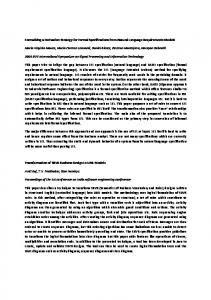
M ⇓ (λx.R) λx.R ⇓ λx.R

N ⇓U (M N ) ⇓ V

R[U/x] ⇓ V

Fig. 1. Big-step specification of the call-by-value evaluation of the untyped λ-calculus.

∀R [ (abs R) ⇓ (abs R) ] ∀M, N, U, V, R [ M ⇓ (abs R) ∧ N ⇓ U ∧ (R U ) ⇓ V ⊃ (app M N ) ⇓ V ] Fig. 2. Horn clause encoding of call-by-value evaluation. Here, all quantified variables are at syntactic type tm except for R, which is at syntactic type tm → tm.

3

Horn clauses

We illustrate the use of Horn clauses in the specification of operational semantics by presenting examples using the λ-calculus and the π-calculus.

3.1

Call-by-value evaluation

Figure 1 contains a big-step semantic specification of call-by-value evaluation for the λ-calculus. Figure 2 contains the corresponding Horn clause encoding of the inference rules in Figure 1. The (infix) predicate symbol ⇓ is a type tm → tm → o and the variable R is of higher-order syntactic type tm → tm. The encoding of the atomic evaluation judgment R[U/x] ⇓ V in Figure 1 is simply (R U ) ⇓ V in Figure 2: that is, the logic expression simply forms the expression (R U ) and once R is instantiated with a λ-abstractions, the logic’s built-in treatment of β-reduction performs the necessary substitution.

3.2

Specifying the pi-calculus α

The relation of one-step (late) transition [28] for the π-calculus is denoted by P −−→ Q, where P and Q are processes and α is an action. The kinds of actions are the silent action τ , the free input action xy, the free output action x ¯y, the bound input action x(y), and the bound output action x ¯(y). The name y in x(y) and x ¯(y) is a binding occurrence. An action without binding occurrences of names is a free action; otherwise it is a bound action. Notice also that we have allowed universal quantifiers to appear in the body of the Horn clauses: these quantifiers are natural complements of allowing λ-binders within terms. ·

The one-step transition relation is represented using two predicates: · −−→ · is of type p → a → p → o and encodes transitions involving the silent and free ·

actions and · −− · is of type p → (n → a) → (n → p) → o and encodes transitions involving bound values. One-step transition judgments are translated to atomic

154

D. Miller / Electronic Notes in Theoretical Computer Science 246 (2009) 147–165 τ

tau:



⊃ τ P −−→ P

in:



⊃ in X M −− M

out:



⊃ out x y P −−→ P

↓X

↑xy

A

A

P −−→ Q

match:

⊃ [x = x]P −−→ Q

A

A

P −− Q

⊃ [x = x]P −− Q

A

A

A

A

A

A

sum: P −−→ R ∨ Q −−→ R ⊃ P + Q −−→ R P −− R ∨ Q −− R ⊃ P + Q −− R A

A

P −−→ P 

par:

⊃ P | Q −−→ P  | Q

A

A

Q −−→ Q

⊃ P | Q −−→ P | Q

A

A

P −− M

⊃ P | Q −− λn(M n | Q)

A

Q −− N. res:

A

∀n(P n −−→ Qn) A

∀n(P n −− P  n) open:

↑Xy

∀y(M y −−→ M  y)

A

⊃ P | Q −− λn(P | N n) A

⊃ νn.P n −−→ νn.Qn A

⊃ νn.P n −− λm νn.P  nm ↑X

⊃ νy.M y −− M 

↓X

↑X

τ

↑X

↓X

τ

↓X

↑XY

τ

↑XY

↓X

τ

close: P −− M ∧ Q −− N ⊃ P | Q −−→ νy.(M y | N y) P −− M ∧ Q −− N ⊃ P | Q −−→ νy.(M y | N y) com: P −− M ∧ Q −−→ Q ⊃ P | Q −−→ M Y | Q P −−→ P  ∧ Q −− N ⊃ P | Q −−→ P  | N Y Fig. 3. The late transition system of the π-calculus as Horn clauses.

formulas as follows (we overload the symbol [[.]] from Section 2.3). xy

↓xy

x ¯y

↑xy

τ

τ

[[P −−→ Q]] = [[P]] −−→ [[Q]] [[P −−→ Q]] = [[P]] −−→ [[Q]]

x(y)

↓x

x ¯(y)

↑x

[[P −−→ Q]] = [[P]] −− λy.[[Q]] [[P −−→ Q]] = [[P]] −− λy.[[Q]]

[[P −−→ Q]] = [[P]] −−→ [[Q]] Figure 3 contains a set of Horn clauses, called Dπ , that encodes the operational semantics of the late transition system for the finite π-calculus. In this specification, free variables are schema variables that are assumed to be universally quantified over the Horn clause in which they appear. These schema variables have primitive types such as a, n, and p as well as functional types such as n → a and n → p. Notice that, as a consequence of using λ-tree syntax for this specification, the usual side conditions in the original specifications of the π-calculus [28] are no

D. Miller / Electronic Notes in Theoretical Computer Science 246 (2009) 147–165

155

longer present. For example, the side condition that X = y in the open rule is implicit, since X is outside the scope of y and therefore cannot be instantiated with y (substitutions into logical expressions cannot capture bound variable names). The adequacy of our encoding is stated in the following proposition (the proof of this proposition can be found in [36]). Proposition 3.1 Let P and Q be processes and α an action. Let n ¯ be a list of free α names containing the free names in P, Q, and α. The transition P −−→ Q is derivable α in the π-calculus if and only if ∀¯ n.[[P −−→ Q]] is provable from the logical theory Dπ . The clauses in Figure 3 come from [25] except that the ∇-quantifier used in that other paper is replaced here by the ∀-quantifier: as is argued in [25], as long as “positive” properties (such as reachability) are computed, the ∇-quantifier can be confused with the ∀ quantifier in the body of Horn clauses.

4

Binary clauses

The reduced class of Horn clause, called binary clauses, can play an important role in modeling computation. As we argue below, they can be used to explicitly order computations whose order is left unspecified in Horn clauses: such an explicit ordering is important if one wishes to use the framework of big-step semantics to capture side-effects and concurrency. They can also be used to capture the notion of abstract machines, a common device for specifying operational semantics. 4.1

Continuation passing in logic programming

Continuation-passing style specifications are possible in logic programming using quantification over the type of formulas [35]. In fact, it is possible to “cps transform” arbitrary Horn clauses into binary clauses as follow. First, for every predicate p of type τ1 → . . . → τn → o (n ≥ 0), we provide a second predicate pˆ of type τ1 → . . . → τn → o → o: that is, an additional argument of type o (the type of formulas) is added to predicate p. Thus, the atomic formula A of the form p t1 . . . tn ) of type (p t1 . . . tn ) is similarly transformed to the formula Aˆ = (ˆ o → o. Using these conventions, the cps transformation of the formula ∀z1 . . . ∀zm [(A1 ∧ . . . ∧ An ) ⊃ A0 ]

(m ≥ 0, n > 0)

is the binary clause ∀z1 . . . ∀zm ∀k [(Aˆ1 (Aˆ2 (· · · (Aˆn k) · · ·))) ⊃ (Aˆ0 k)]. Similarly, the cps transformation of the formula ∀z1 . . . ∀zm [A0 ]

is

∀z1 . . . ∀zm ∀k [k ⊃ (Aˆ0 k)].

If P is a finite set of Horn clauses and Pˆ is the result of applying this cps transformation to all clauses in P, then P A if and only if Pˆ (Aˆ ).

156

D. Miller / Electronic Notes in Theoretical Computer Science 246 (2009) 147–165

((M ⇓ (abs R)) ; (N ⇓ U ) ; ((R U ) ⇓ V ) ; K) ⊃ ((app M N ) ⇓ V ) ; K (((abs R) ⇓ (abs R)) ; K) ⊃ K. Fig. 4. Binary version of call-by-value evaluation.

Consider again the presentation of call-by-value evaluation given by the Figure 2. In order to add side-effecting features, this specification must be made more explicit: in particular, the exact order in which M , N , and (R U ) are evaluated must be specified. The cps transformation of that specification is given in Figure 4: there, evaluation is denoted by a ternary predicate of type tm → tm → o → o which is written using both the ⇓ arrow and a semicolon: e.g., the relation “M evaluates to V with the continuation K” is denoted by (M ⇓ V ) ; K. In this specification, goals are now sequenced in the sense that bottom-up proof search is forced to construct a proof of one evaluation pair before others such pairs. Of course, in this setting, any ordering works, so it is possible to prove the following: the goal ((M ⇓ V ) ; ) is provable if and only if V is the call-by-value result of M . The order in which evaluation is executed is now forced not by the use of logical connectives but by the use of the non-logical constant (· ⇓ ·) ; ·. 4.2

Abstract Machines

Abstract machines, which are often used to specify operational semantics, can be encoded naturally using binary clauses. To see this, consider the following definition of Abstract Evaluation System (AES) which generalizes the notion of abstract machines [12]. Recall that a term rewriting system is a pair (Σ, R) such that Σ is a signature and R is a set of directed equations {li ⇒ ri }i∈I with li , ri ∈ TΣ (X) and V(ri ) ⊆ V(li ). Here, TΣ (X) denotes the set of first-order terms with constants from the signature Σ and free variables from X, and V(t) denotes the set of free variables occurring in t. An abstract evaluation system is a quadruple (Σ, R, ρ, S) such that the pair (Σ, R ∪ {ρ}) is a term rewriting system, ρ is not a member of R, and S ⊆ R. Evaluation in an AES is a sequence of rewriting steps with the following restricted structure. The first rewrite rule must be an instance of the ρ rule. This rule can be understood as “loading” the machine to an initial state given an input expression. The last rewrite step must be an instance of a rule in S: these rules denote the successful termination of the machine and can be understood as “unloading” the machine and producing the answer or final value. All other rewrite rules are from R. We also make the following significant restriction to the general notion of term rewriting: all rewriting rules must be applied to a term at its root. This restriction significantly simplifies the computational complexity of applying rewrite rules during evaluation in an AES. A term t ∈ TΣ (∅) evaluates to the term s (with respect to the AES (Σ, R, ρ, S)) if there is a series of rewriting rules satisfying the restrictions above that rewrites t into s. The SECD machine [16] and Krivine machine [8] are both AESs and variants of

157

D. Miller / Electronic Notes in Theoretical Computer Science 246 (2009) 147–165

M

⇒



nil,

M,

nil 



E,

λM ,

X :: S

⇒

X :: E,

M,

S



E,

M ˆN,

S

⇒



E,

M,

{E, N } :: S

{E  , M } :: E,

0,

S

⇒



E,

M,

S



E,

n,

S



X :: E,

n + 1,

S

⇒



E,

λM ,

nil 

⇒

{E, λM }

M

⇒

nil, nil, M :: nil, nil 

S, E, λM :: C, D

⇒

{E, λM } :: S, E, C, D

S, E, (M ˆ N ) :: C, D

⇒

S, E, M :: N :: ap :: C, D

S, E, n :: C, D

⇒

nth(n, E) :: S, E, C, D

X :: {E  , λM } :: S, E, ap :: C, D ⇒ nil, X :: E  , M :: nil, (S, E, C) :: D X :: S, E, nil, (S  , E  , C  ) :: D ⇒ X :: S, E, nil, nil

⇒

X :: S  , E  , C  , D

X

Fig. 5. The Krivine machine (top) and SECD machine (bottom).

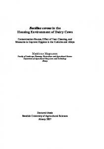
these are given in Figure 5. There, the syntax for λ-terms uses de Bruijn notation with ˆ (infix) and λ as the constructors for application and abstraction, respectively, and {E, M } denotes the closure of term M with environment E. The first rule given for each machine is the “load” rule or ρ of their AES description. The last rule given for each is the “unload” rule. (In each of these cases, the set S is a singleton.) The remaining rules are state transformation rules, each one moving the machine through a computation step. A state in the Krivine machine is a triple E, M, S in which E is an environment, M is a single term to be evaluated and S is a stack of arguments. A state in the SECD machine is a quadruple S, E, C, D in which S is a stack of computed values, E is an environment (here just a list of terms), C is a list of commands (terms to

158

D. Miller / Electronic Notes in Theoretical Computer Science 246 (2009) 147–165

unload t unload t unload t rewrite sn .. . unload t rewrite si .. . unload t rewrite s1 unload t load s Fig. 6. A proof related to the execution of an abstract machine.

be evaluated) and D is a dump or saved state. The expression nth(n, E), used to access variables in an environment, is treated as a function that returns the n + 1st element of the list E. Although Landin’s original description of the SECD machine used variables names, our use of de Bruijn numerals does not change the essential mechanism of that machine. There is a natural and immediate way to see a given AES as a set of binary clauses. Let load, unload, and rewrite be three predicates of one argument each. Given the AES (Σ, R, ρ, S) let B be the set of binary clauses composed of the following three kinds of formulas: ∀ˆ x [rewrite r ⊃ load l] where ρ is the rewrite rule l ⇒ r, one clause of the form ∀ˆ x [rewrite r ⊃ rewrite l] for every rewrite rule l ⇒ r in R, and one clause of the form ∀ˆ x [unload r ⊃ rewrite l] for every rewrite rule l ⇒ r in S. It is then easy to show that if we start with term t and evaluate to s (this can be a non-deterministic relationship) then from the set of clauses B we can prove unload t ⊃ load s. In particular, if this implication is provable from B then it has a proof of the form displayed in Figure 6. The transitions of the abstract machine can be read directly from this proof: given the term s, the machine’s state is initialized to be s1 , which is then repeatedly rewritten yielding the sequence of terms s2 , . . . , sn , at which point the machine is unloaded to get the value t. For more about translating SOS specifications directly into abstract machines, see [12]. In order to motivate our next operational semantic framework, consider the problem of specifying side-effects, exceptions, and concurrent (multi-threaded) computation with binary clauses. Since all the dynamics of computation is represented via term structures (say, within s, s1 , . . . , sn , t) all the information about these threads, reference cells, exceptions, etc., must be maintained as, say, lists within these other terms. Such an approach to specifying these features of a programming language lacks modularity and makes little use of logic. We now consider extending binary clauses so that these additional features have a much more natural and modular specification.

5

Linear logic

We now illustrate how linear logic can be used to capture multiset rewriting. Given that many aspects of computation can be captured using multiset rewriting, it is possible to describe a subset of linear logic that includes binary clauses but provides

D. Miller / Electronic Notes in Theoretical Computer Science 246 (2009) 147–165

159

a natural means to capture side effects and concurrency. The examples in this section are adapted from [22]. 5.1

Capturing multiset rewriting

The right-hand-side of a sequent in linear logic is a multiset of formula. At the formula level, the  connective of linear logic (the multiplicative disjunction and the de Morgan dual of ⊗) can be used to build multisets. For example, the propositional formula a  b  b  a  c can be seen as an encoding of the multiset that contains two occurrences of a, two occurrences of b, one occurrence of c, and no occurrences of any other formulas. The unit for , written as ⊥, encodes the empty multiset. A suitable generalization of backchaining in linear logic can be used to formulate rewriting of that multiset. To illustrate this connection between rewriting and backchaining, assume that Δ is a set of linear logic formulas that contains the formula c  d  e −◦ a  b. (The  symbol binds tighter than −◦.) Consider also the sequent ! Δ −→ a, b, Γ. A proof for this sequent that backchains on the clause above looks like the following. ! Δ −→ c, d, e, Γ R ! Δ −→ c, d  e, Γ a −→ a b −→ b R L ! Δ −→ c  d  e, Γ a  b −→ a, b −◦L ! Δ, c  d  e −◦ a  b −→ a, b, Γ !D ! Δ −→ a, b, Γ When we read this proof fragment bottom-up, we can see that the action of selecting the displayed formula above and doing a focused set of introductions (a.k.a. backchaining) on it causes the multiset on the right-hand side to be rewritten from a, b, Γ to c, d, e, Γ. 5.2

Adding a counter to evaluation

Consider again the binary clause example given in Figure 4. First, it is easy to show that in Horn clauses in general, the top-level intuitionistic implication ⊃ can be rewritten as the linear implication −◦ without changing the operational reading of proof search [13]. With this change, the binary clauses in that figure are also an example of multiset rewriting: in this occasion, one atom is repeatedly replace by another atom (until the atom is replaced by a final continuation). In this way, binary clauses can be seen as modeling single-threaded computation. Now that we have embedded binary clauses within the richer setting of linear logic, it is easy to see how “multi-threaded” computations might be organized. We present a couple of examples here. Consider adding to the untyped λ-calculus a single global counter that can be read and incremented. In particular, we shall place all integers into type tm and add two additional constructors of tm, namely get and inc. The intended operational semantics of these two constants is that evaluating the first returns the current value

160

D. Miller / Electronic Notes in Theoretical Computer Science 246 (2009) 147–165

of the counter and evaluating the second increments the counter’s value and returns the counter’s old value. We also assume that integers are values: that is, for every integer i the clause ∀k(k −◦ (i ⇓ i) ; k) is part of the evaluator’s specification. The multiset rewriting specification of these two additional constructors can be given as the two formulas ∀K∀V (r V  K −◦ ((get ⇓ V ) ; K)  r V ) and ∀K∀V (r (V + 1)  K −◦ ((inc ⇓ V ) ; K)  r V ). Here, the atom of the form (r x) denotes the “r-register” with value x. Let D contain the two formulas in Figure 4, the two formulas displayed above, and the formulas mentioned above describing the evaluation of integers. Then D is a specification of the call-by-value evaluator with one global counter in the sense that the logical judgment ! D ((M ⇓ V ) ; )  r 0 holds exactly when we expect the program M to evaluation to V in the setting when the register r is initialized to 0. Of course, the name of the register should not be a part of the specification of a counter. Fortunately, logic comes equipped with abstraction mechanisms that allow hiding the name of this register. In Figure 7 there are three specifications, E1 , E2 , and E3 , of a counter: all three specifications store the counter’s value in an atomic formula as the argument of the predicate r. In these three specifications, the predicate r is existentially quantified over the specification in which it is used so that the atomic formula that stores the counter’s value is itself local to the counter’s specification (such existential quantification of predicates is a familiar technique for implementing abstract data types in logic programming [19]). The first two specifications store the counter’s value on the right of the sequent arrow, and reading and incrementing the counter occurs via a synchronization between an ⇓-atom and an r-atom. In the third specification, the counter is stored as a linear assumption on the left of the sequent arrow, and synchronization is not used: instead, the linear assumption is “destructively” read and then rewritten in order to specify the get and inc functions (counters such as these are described in [13]). Finally, in the first and third specifications, evaluating the inc symbol causes 1 to be added to the counter’s value. In the second specification, evaluating the inc symbol causes 1 to be subtracted from the counter’s value: to compensate for this unusual implementation of inc, reading a counter in the second specification returns the negative of the counter’s value. Although these three specifications of a global counter are different, they should be equivalent in the sense that evaluation cannot tell them apart. Although there are several ways that the equivalence of such counters can be proved, the specifications of these counters are, in fact, logically equivalent. Proposition. The three entailments E1 E2 , E2 E3 , and E3 E1 are provable in linear logic. The proof of each of these entailments proceeds (in a bottom-up fashion) by

D. Miller / Electronic Notes in Theoretical Computer Science 246 (2009) 147–165

161

E1 = ∃r[ (r 0)⊥ ⊗ ! ∀K∀V (r V  K −◦ ((get ⇓ V ) ; K)  r V ) ⊗ ! ∀K∀V (r (V + 1)  K −◦ ((inc ⇓ V ) ; K)  r V )] E2 = ∃r[ (r 0)⊥ ⊗ ! ∀K∀V (r V  K −◦ ((get ⇓ (−V )) ; K)  r V ) ⊗ ! ∀K∀V (r (V − 1)  K −◦ ((inc ⇓ (−V )) ; K)  r V )] E3 = ∃r[ (r 0) ⊗ ! ∀K∀V (r V ⊗ (r V −◦ K) −◦ ((get ⇓ V ) ; K)) ⊗ ! ∀K∀V (r V ⊗ (r (V + 1) −◦ K) −◦ ((inc ⇓ V ) ; K))] Fig. 7. Three specifications of a global counter.

choosing an eigen-variable to instantiate the existential quantifier on the left-hand side and then instantiating the right-hand existential quantifier with some term involving that eigen-variable. Assume that in all three cases, the eigen-variable selected is the predicate symbol s. Then the first entailment is proved by instantiating the right-hand existential with λx.s (−x); the second entailment is proved using the substitution λx.(s (−x))⊥ ; and the third entailment is proved using the substitution λx.(s x)⊥ . The proof of the first two entailments must also use the identities −0 = 0, −(x + 1) = −x − 1, and −(x − 1) = −x + 1. The proof of the third entailment requires no such identities. Clearly, logical equivalence is a strong equivalence: it immediately implies that evaluation cannot tell the difference between any of these different specifications of a counter. For example, assume E1 (M ⇓ V ) ; . Then by the cut inference rule (modus ponens) and the above proposition, we have E2 (M ⇓ V ) ; . It is possible to generalize a bit the previous example involving a single global counter to languages that have the ability to generate references dynamically, much as one finds in, say, Algol or Standard ML [6,22].

5.3

Specification of Concurrency primitives

Following [22], we show how concurrency primitives inspired by those found in Concurrent ML (CML) [33] can be specified in linear logic: we assume that the reader has some familiarity with this extension to ML.

162

D. Miller / Electronic Notes in Theoretical Computer Science 246 (2009) 147–165

K −◦ (none ⇓ none) ; K. (E ⇓ V ) ; K −◦ ((guard E) ⇓ (guard V )) ; K. (E ⇓ V ) ; K −◦ ((poll E) ⇓ (poll V )) ; K. (E ⇓ V ) ; K −◦ ((receive E) ⇓ (receive V )) ; K. (E ⇓ V ) ; K −◦ ((some E) ⇓ (some V )) ; K. (E ⇓ U ) ; ((F ⇓ V ) ; K) −◦ ((choose E F ) ⇓ (choose U V )) ; K. (E ⇓ U ) ; ((F ⇓ V ) ; K) −◦ ((transmit E F ) ⇓ (transmit U V )) ; K. (E ⇓ U ) ; ((F ⇓ V ) ; K) −◦ ((wrap E F ) ⇓ (wrap U V )) ; K. Fig. 8. These CML-like constructors evaluate to themselves.

Consider extending the untyped λ-calculus with the following constructors. none : tm. guard, poll, receive, some, sync : tm → tm. choose, transmit, wrap : tm → tm → tm. spawn, newchan : (tm → tm) → tm. The meaning of these constructors is then given using the linear logic formulas in Figures 8 and 9. The clauses in Figures 8 specify the straightforward evaluation rules for the eight data constructors. In Figure 9, the predicate event is of type tm → tm → o → o and is used to store in the multiset “events”, a technical aspect of this semantic specification. The first three clauses of that figure defined the meaning of the three special forms sync, spawn, and newchan. The remaining clauses specify the event predicate. The formulas in Figure 9 allow for multiple threads of evaluation. Evaluation of the spawn function initiates a new evaluation thread. The newchan function causes a new eigenvariable to be picked (via the ∀c quantification) and then to assume that that eigen-variable is a value (via the assumption ∀I(I −◦ (c ⇓ c) ; I)): such a new value can be used to designate new channels for use in synchronization (the clause for newchan is not strictly speaking a Horn clause). The sync primitive allows for synchronization between threads: its use causes an “evaluation thread” to become an “event thread.” The behaviors of event threads are described by the remaining clauses in Figure 9. The primitive events are transmit and receive and they represent two halves of a synchronization between two event threads. Notice that the clause describing their meaning is the only clause in Figure 9 that has a head with more than one atom. The non-primitive events choose, wrap, guard, and poll are reduced to other calls to event and ⇓. The choice event is implemented as a local, non-deterministic choice. (Specifying global choice, as in CCS [27], would be much more involved.) The wrap and guard events chain together evaluation and

D. Miller / Electronic Notes in Theoretical Computer Science 246 (2009) 147–165

163

eval E U (event U V K) −◦ ((sync E) ⇓ V ) ; K. (((R unit) ⇓ unit) ; ⊥)  K −◦ ((spawn R) ⇓ unit) ; K. ∀c(∀I(I −◦ (c ⇓ c) ; I) ⊃ ((R c) ⇓ V ) ; K) −◦ ((newchan R) ⇓ V ) ; K. K  L −◦ event (receive C) V K  event (transmit C V ) unit L event E V K −◦ event (choose E F ) V K. event F V K −◦ event (choose E F ) V K. event E U (((app F U ) ⇓ V ) ; K) −◦ event (wrap E F ) V K. ((app F unit) ⇓ U ) ; (event U V K) −◦ event (guard F ) V K. (event E U ) & K −◦ event (poll E) (some E) K. K −◦ event (poll E) none K. Fig. 9. Specifications of some primitives similar to those in Concurrent ML.

synchronization but in direct orders. The only use of additive linear logic connectives, in particular & and , in any of our semantic specifications is in the specification of polling: in an attempt to synchronize with (poll E) (with the continuation K) the goal (event E U ) & K is attempted (for some unimportant term U ). Thus, a copy of the current evaluation threads is made and (event E U ) is attempted in one of these copies. This atom is provable if and only if there is a complementary event for E in the current environment, in which case, the continuation  brings us to a quick completion and the continuation K is attempted in the original and unspoiled context of threads. If such a complementary event is not present, then the other clause for computing a polling event can be used, in which case, the result of the poll is none, which signals such a failure. The semantics of polling, unfortunately, is not exactly as intended in CML since it is possible to have a polling event return none even if the event being tested could be synchronized. This analysis of polling is similar to the analysis of testing in process calculus as described in [21]. The PhD thesis of Chirimar [6] presents a linear logic specification of a programming language motivated by Standard ML [29]. In particular, a specification for the call-by-value λ-calculus is provided, and then modularly extended with the specifications of references, exceptions, and continuations: each of these features is specified without complicating the specifications of other the features.

6

Conclusion

There is a lot of interest in being able to reason about operational semantic descriptions of programming languages: see, for example, the POPLmark challenge [1], and the long-standing research efforts using dependently typed λ-calculus [30] and certain higher-order logics [2,18,25]. In this paper, we have tried to describe one ap-

164

D. Miller / Electronic Notes in Theoretical Computer Science 246 (2009) 147–165

proach to formally specifying operational semantics so that such verification efforts have a solid foundation. We have provided such a foundation by encoding three different formalisms–SOS, abstract machines, and multiset rewriting—into collections of logic formulas. The theory of proofs can then be used to provide completely formal meaning to such specifications. Acknowledgments. I would like to thank Andrew Gacek for providing several useful comments on an earlier draft of this paper.

References [1] Aydemir, B. E., A. Bohannon, M. Fairbairn, J. N. Foster, B. C. Pierce, P. Sewell, D. Vytiniotis, G. Washburn, S. Weirich and S. Zdancewic, Mechanized metatheory for the masses: The POPLmark challenge, in: Theorem Proving in Higher Order Logics: 18th International Conference, number 3603 in LNCS (2005), pp. 50–65. [2] Baelde, D., A. Gacek, D. Miller, G. Nadathur and A. Tiu, The Bedwyr system for model checking over syntactic expressions, in: F. Pfenning, editor, 21th Conference on Automated Deduction (CADE), number 4603 in LNAI (2007), pp. 391–397. URL http://www.lix.polytechnique.fr/Labo/Dale.Miller/papers/cade2007.pdf [3] Banˆ atre, J.-P. and D. L. M´ etayer, Programming by Multiset Transformation, Communications of the ACM 36 (1993), pp. 98–111. [4] Berry, G. and G. Boudol, The chemical abstract machine, Theoretical Computer Science 96 (1992), pp. 217–248. [5] Bistarelli, S., I. Cervesato, G. Lenzini and F. Martinelli, Relating multiset rewriting and process algebras for security protocol analysis, Journal of Computer Security 13 (2005), pp. 3–47. [6] Chirimar, J., “Proof Theoretic Approach to Specification Languages,” Ph.D. thesis, University of Pennsylvania (1995). URL http://www.lix.polytechnique.fr/Labo/Dale.Miller/chirimar/phd.ps [7] Church, A., A formulation of the simple theory of types, J. of Symbolic Logic 5 (1940), pp. 56–68. [8] Curien, P.-L., The λρ-calculus: An abstract framework for environment machines, Technical report, LIENS–CNRS (1990). [9] Gordon, M. J. C., “Programming Language Theory and its Implementation,” Prentice Hall, 1988. [10] Gunter, C. A., “Semantics of Programming Languages: Structures and Techniques,” Foundations of Computing, MIT Press, 1992. [11] Gurevich, Sequential abstract-state machines capture sequential algorithms, ACM Trans. on Computational Logic 1 (2000), pp. 77–111. [12] Hannan, J. and D. Miller, From operational semantics to abstract machines, Mathematical Structures in Computer Science 2 (1992), pp. 415–459. [13] Hodas, J. and D. Miller, Logic programming in a fragment of intuitionistic linear logic, Information and Computation 110 (1994), pp. 327–365. [14] Kahn, G., Natural semantics, in: Proceedings of the Symposium on Theoretical Aspects of Computer Science, LNCS 247 (1987), pp. 22–39. [15] Kanovich, M. I., Petri nets, Horn programs, Linear Logic and vector games, Annals of Pure and Applied Logic 75 (1995), pp. 107–135. [16] Landin, P. J., The mechanical evaluation of expressions, Computer Journal 6 (1964), pp. 308–320. [17] McCarthy, J., Towards a mathematical science of computation, in: C. M. Popplewell, editor, Information Processing, North-Holland, 1963 pp. 21–28. [18] McDowell, R. and D. Miller, Reasoning with higher-order abstract syntax in a logical framework, ACM Trans. on Computational Logic 3 (2002), pp. 80–136.

D. Miller / Electronic Notes in Theoretical Computer Science 246 (2009) 147–165

165

[19] Miller, D., Lexical scoping as universal quantification, in: Sixth International Logic Programming Conference (1989), pp. 268–283. URL http://www.lix.polytechnique.fr/Labo/Dale.Miller/papers/iclp89.pdf [20] Miller, D., Proof theory as an alternative to model theory, Newsletter of the Association for Logic Programming (1991), guest editorial. URL http://www.lix.polytechnique.fr/Labo/Dale.Miller/papers/ProofTheoryAsAlternative.html [21] Miller, D., The π-calculus as a theory in linear logic: Preliminary results, in: E. Lamma and P. Mello, editors, 3rd Workshop on Extensions to Logic Programming, number 660 in LNCS (1993), pp. 242–265. URL http://www.lix.polytechnique.fr/Labo/Dale.Miller/papers/pic.pdf [22] Miller, D., Forum: A multiple-conclusion specification logic, Theoretical Computer Science 165 (1996), pp. 201–232. [23] Miller, D., Abstract syntax for variable binders: An overview, in: J. Lloyd and et. al., editors, Computational Logic - CL 2000, number 1861 in LNAI (2000), pp. 239–253. URL http://www.lix.polytechnique.fr/Labo/Dale.Miller/papers/ltrees.pdf [24] Miller, D., G. Nadathur, F. Pfenning and A. Scedrov, Uniform proofs as a foundation for logic programming, Annals of Pure and Applied Logic 51 (1991), pp. 125–157. [25] Miller, D. and A. Tiu, A proof theory for generic judgments, ACM Trans. on Computational Logic 6 (2005), pp. 749–783. [26] Milner, R., “A Calculus of Communicating Systems,” LNCS 92, Springer-Verlag, New York, NY, 1980. [27] Milner, R., “Communication and Concurrency,” Prentice-Hall International, 1989. [28] Milner, R., J. Parrow and D. Walker, A calculus of mobile processes, Part II, Information and Computation (1992), pp. 41–77. [29] Milner, R., M. Tofte and R. Harper, “The Definition of Standard ML,” MIT Press, 1990. [30] Pfenning, F. and C. Sch¨ urmann, System description: Twelf — A meta-logical framework for deductive systems, in: H. Ganzinger, editor, 16th Conference on Automated Deduction (CADE), number 1632 in LNAI (1999), pp. 202–206. [31] Plotkin, G., A structural approach to operational semantics, DAIMI FN-19, Aarhus University, Aarhus, Denmark (1981). [32] Plotkin, G. D., The origins of structural operational semantics, J. of Logic and Algebraic Programming 60 (2004), pp. 3–15. [33] Reppy, J. H., CML: A higher-order concurrent language, in: ACM SIGPLAN Conference on Programming Language Design and Implementation, 1991, pp. 293–305. [34] Stoy, J. E., “Denotational Semantics: The Scott-Strachey Approach to Programming Language Theory,” MIT Press, Cambridge, MA, 1977. [35] Tarau, P., Program transformations and WAM-support for the compilation of definite metaprograms, in: Proceedings of the First and Second Russian Conference on Logic Programming, number 592 in LNAI (1992), pp. 462–473. [36] Tiu, A., “A Logical Framework for Reasoning about Logical Specifications,” Ph.D. thesis, Pennsylvania State University (2004). URL http://etda.libraries.psu.edu/theses/approved/WorldWideIndex/ETD-479/