Department of Neuroscience, Division of Human Brain Research. Karolinska .... ure 1 shows a summary of an evaluation of this processing stage, by computing.
Fully Automatic Segmentation of MRI Brain Images using Probabilistic Anisotropic Diffusion and Multi-Scale Watersheds� Carl Undeman1,2 and Tony Lindeberg1 1
Computational Vision and Active Perception Laboratory (CVAP) Department of Numerical Analysis and Computer Science KTH, SE-100 44 Stockholm, Sweden
2
Department of Neuroscience, Division of Human Brain Research Karolinska Institutet, SE-171 77 Solna, Sweden
Abstract. This article presents a fully automatic method for segmenting the brain from other tissue in a 3-D MR image of the human head. The method is a an extension and combination of previous techniques, and consists of the following processing steps: (i) After an initial intensity normalization, an affine alignment is performed to a standard anatomical space, where the unsegmented image can be compared to a segmented standard brain. (ii) Probabilistic diffusion, guided by probability measures between white matter, grey matter and cerebrospinal fluid, is performed in order to suppress the influence of extra-cerebral tissue. (iii) A multi-scale watershed segmentation step creates a slightly oversegmented image, where the brain contour constitutes a subset of the watershed boundaries. (iv) A segmentation of the over-segmented brain is then selected by using spatial information from the pre-segmented standard brain in combination with additional stages of probabilistic diffusion, morphological operations and thresholding. The composed algorithm has been evaluated on 50 T1-weighted MR volumes, by visual inspection and by computing quantitative measures of (i) the similarity between the segmented brain and a manual segmentation of the same brain, and (ii) the ratio of the volumetric difference between automatically and manually segmented brains relative to the volume of the manually segmented brain. The mean value of the similarity index was 0.9961 with standard deviation 0.0034 (worst value 0.9813, best 0.9998). The mean percentage volume error was 0.77 % with standard deviation 0.69 % (maximum percentage error 3.81 %, minimum percentage error 0.05 %).
1
Introduction
Segmenting the brain from other tissue in a 3-D MR image of the human head is an important pre-processing stage for many tasks, for example: �
Shortened version in L. Griffin and M. Lillholm (Eds), Proc. Scale-Space’03 , Isle of Skye, Scotland, Springer Lecture Notes in Computer Science, volume 2695, 641–656.
2
– when aligning individual brains to a standard anatomical format, – when delimiting a volume in the brain where statistical measurements of brain activation are to be performed, and – when computing morphological measures of the shape of the brain. Until recently, high-quality segmentation was carried out semi-automatically at our laboratory, which implied a large amount of manual intervention. The purpose of this article is to develop a procedure for carrying out this task in a fully automatic manner. This automation step is also important for the development of brain databases containing functional brain activation images as well as procedures for analyzing such data in a fully automated manner. Despite the fact that the MR imaging technique provides images with high spatial resolution and good soft-tissue contrast, computing a high-quality and fully automatic segmentation of the brain from other tissue is a non-trivial problem. Some reasons why the problem is hard, are imperfections in the data due to electrical and thermal noise, errors in the scanner due to inhomogeneities in the magnetic field, partial volume effects and biological variations between subjects. To address this problem, we propose a multi-stage solution that combines and extends earlier image processing methods, essentially based on: – an approximate normalization to standard anatomical format, so that anatomical information from a pre-segmented standard brain can be exploited, – an anisotropic diffusion algorithm, guided by approximate probabilities for different types of tissue, in order to improve the performance of subsequent multi-scale watershed segmentation and morphological processing. The integrated algorithm has been evaluated on 50 T1-weighted MR images of the human head, which were also segmented manually (see section 4). In addition, the algorithm has been applied to at least 200 more brain images, with highly successful results.
2
Approaches to brain segmentation
To address the brain segmentation problem, several different types of approaches have been considered in the literature. Since the brain consists of a known set of tissue types (mainly white matter, grey matter, bone and cerebrospinal fluid) a natural first approach consists of capturing the distributions of these tissues, and aiming at a classification from the intensity values, see for example (Atkins & Mackiewich 1997), who fitted a mixture of Rayleigh distributions to the histogram of the original MR image. The main strength of this method is that it allows for fast and easy implementation. The main weakness is that the distributions of the different tissue types in general overlap, which means that it will not be possible to find thresholds that separate brain and non-brain tissue. Another approach is to align a pre-segmented template brain to the brain of any individual subject, and thereby propagate the segmentation to this subject. Such an approach has been used by (Collins et al. 1994), (Dawant et al. 1999)
3
and (Holden et al. 2001) for identifying anatomical substructures, and provides an efficient way to incorporate anatomical information into segmentation algorithms. These works, however, depend on high quality registration between the template brain and the unsegmented brain, which may be hard to obtain. To detect tissue boundaries from local information, edge detection is a natural approach to consider. However, since the contrast may vary substantially in an MR image of a brain, it will in general not be possible to find thresholds and scale levels that lead to connected edges that separate different tissues into connected regions. A more refined approach has been considered by (Zeng et al. 1999), who developed an edge detector aimed at detecting only edges that correspond to boundaries between pre-defined tissue types, e.g. between cerebrospinal fluid and white matter. The method is based on approximating the distribution of tissue types A and B by Gaussian distributions, and then computing the probability pA (x) that a voxel x belongs to tissue A, and the probability pB (N (x)) that a neighbour N (x) of x belongs to tissue type B. The product pA (x) pB (N (x)) will only assume high values when both the factors are high, and in this way the probability of a border between any two tissue types can be estimated. Another limitation of edge detection preceded by Gaussian smoothing is that edges with low contrast may be lost during the smoothing operation and that highly curved edges may be rounded. To address these issues, several anisotropic diffusion schemes have been developed, where the Gaussian smoothing operator is replaced by an edge preserving anisotropic diffusion step, see e.g. (ter Haar Romeny 1994, Weickert 1998) for overviews and (Gerig et al. 1992) for an application to brain segmentation. More specific multi-scale methods have also been developed. By extending the ideas of multi-scale extrema linking (Koenderink 1984, Lifshitz & Pizer 1990, Lindeberg 1994), (Olsen 1997) developed a multi-scale watershed approach based on the definition of sinks in the gradient magnitude map at all scales in a Gaussian scale-space representation of the original image. Provided that an appropriate scale level can be selected, this approach can be expected to give rise to an over-segmentation of the anatomical MR image, where the boundaries of the brain constitute a subset of the boundaries of the watersheds computed from the gradient magnitude image. By linking the watershed segments between different scales, a coarse scale segmentation can be propagated to finer scales by following links over scales. In continued work by (Dam & Nielsen 2000), non-linear diffusion was added as a complement. As far as we know, however, these methods have not been fully automated, and require a certain degree of operator assistance. An interesting alternative in the area of automated watershed approaches has been presented by (Hahn & Peitgen 2000), based on a modified watershed transform. Linking of image structures over scales has been considered also (Vincken et al. 1997) by establishing probabilistic links between image structures over scales, and then propagating a coarse-scale segmentation to finer scales in a probabilistic manner. A combination of probabilistic relations and anisotropic diffusion referred to as probabilistic diffusion has been presented by (Arridge
4
& Simmons 1997), based on the idea of using probabilities of different classes to control the conductance in a diffusion equation, as opposed to intensity differences. In close relation to these notions, three-dimensional Markov random field models have been developed by e.g. (Rajapakse et al. 1997) and (Held et al. 1997). Moreover, morphological processing is used in several works (Atkins & Mackiewich 1997, Lemieux et al. 1999). For further overviews of brain segmentation, see e.g. (Atkins & Mackiewich 1997) and (Hahn & Peitgen 2000).
3
Proposed method
Based on the abovementioned literature survey, we propose to address the problem of segmenting MR images of human brains using a combination of the following types of methods: – Empirically, we have found that MR images often contain spurious high values. To reduce the possibly negative influence of these, an intensity normalization will be performed as a first step in the proposed algorithm. – A spatial normalization is a natural pre-processing step, since using a presegmented standard brain, prior knowledge about the shape of the brain can be effectively represented by transforming the given image into a standard anatomical space. – We will make use of probabilistic anisotropic diffusion guided by edges between different types of tissue as an important pre-processing stage to multiscale watershed segmentation. Probabilistic anisotropic diffusion may also be used for reducing the negative influence of inhomogeneities in the unsegmented image. – Multi-scale watershed segmentation transforms the image into a collection of volumetric elements. Identifying the volumetric elements that constitute the brain can be accomplished by using prior anatomical knowledge obtained via the spatial normalization step. – Post-processing using a combination of probabilistic anisotropic diffusion, morphological operations and thresholding for computing the final result. In the following we will describe each method and show that a highly useful method for brain segmentation can be obtained by combining these modules in the proposed novel way. 3.1
Intensity normalization
To avoid the possibly negative influence of spurious high values in the original MR image, an intensity normalization was performed prior to the affine normalization. This intensity normalization was carried out by estimating a central region of the brain, by computing the weighted center of gravity in the MR image, and computing mean and standard deviation of the intensity values in the central region. A high threshold was chosen two standard deviations above the mean value in the central region, and each voxel having an intensity value above the high threshold was set to this value.
5
3.2
Spatial normalization by affine warping
To transform the brain images to a standard anatomical space, we apply an affine transformation in 3-D which in practice is computed using the AIR package (Woods et √ al. 1998) with a 12 parameter model and a 6 mm Gaussian FWHM (FWHM = 2σ 2 ln 2) pre-filtering of both the target and the input image. Figure 1 shows a summary of an evaluation of this processing stage, by computing the intersection of 50 manually segmented brains that were transformed to a standard anatomical space in this way. As can be seen, this processing stage effectively reduces the main variations in brain anatomy between different subjects. Certain individual variations, however, remain, which leads to the need for more refined processing stages that will be described next.
Fig. 1: The contour of the intersection of 50 stripped brains, linearly transformed to the standard brain, compared to the binary standard brain mask. (a) a sagittal slice, (b) a coronal slice (b), (c)–(d) two horizontal views.
3.3
Capturing the intensity distributions of different tissues
Due to the alignment of the input image to a standard anatomical brain, we can use a manual pre-segmentation of the standard brain into different tissue types (white matter, grey matter, cerebrospinal fluid and bone) as an initial estimate of the segmentation that is to be computed. In particular, since the volume of the transformed brain ideally will be equal to the volume of the standard brain, we can initially assume that the volume of white matter, grey matter and cerebrospinal fluid is equal in these two brains. Thus, threshold values for each tissue type can be easily computed from the idea of sorting the voxels in the transformed brain image, and assuming that the intensities are ordered LCSF < LGM < LW M < LBON E (for simplicity we denote both bone, eye muscles and vascular tissue by “bone”). If the volume of cerebrospinal fluid is VCSF , LCSF can be determined from the lowest VCSF voxels, etc. Due to the fact that some background voxels may be (and often are) included in the support region of the pre-segmented brain mask, the lower threshold LCSF can sometimes be close to the intensity of the background. This is however not a problem since we want to treat background and CSF voxels the same way when
6
Fig. 2: (a) An MR image of a brain after intensity normalization and scaled to values between 0.0 and 100.0. (b) The computed intensity intervals are marked in the histogram: CSF [0.0-36.2], GM [36.2-69.5], WM [69.5-89.6] and BONE [89.6-100.0].
segmenting the brain from surrounding tissue. Moreover, the threshold between white matter and bone, can sometimes be in the bone intensity region, due to the fact that some bone voxels are likely to be included in the support region of the pre-segmented standard brain. Thus, the following modification is used in practice: Every voxel outside the standard brain mask in the transformed image with an intensity above the mean value of the intensity for white matter is taken to be a bone voxel. The low threshold value for the bone voxels is then computed as the average of the mean value for white matter and the mean value for the bone voxels outside the standard brain mask. Figure 2 shows a histogram of an MR image with associated intensity intervals for CSF , GM , W M and BON E determined in this way. 3.4
Multi-scale watershed segmentation
For segmenting an MR image using edge information, it is natural to compute gradient magnitude maps and to associate a watershed with each local minimum. If the watersheds are computed at a too fine scale, however, there will be a large over-segmentation, while if we choose a too coarse scale the boundaries between the watershed regions will not constitute a superset of the boundaries between the different tissue types. Hence, selecting a proper scale level for computing the gradient magnitude is of crucial importance. The selection of reasonable subsets may be simplified by considering coarse-to-fine propagations of watershed support regions, using criteria based on overlap of support regions, intensity levels and inclusion of local minima. Figure 3 shows a few examples of watersheds, computed according to the method in (Vincent & Soille 1991), propagated in this manner. In general, however, it may still be non-trivial to automatically select which watershed regions should be included in the final segmentation. For
7
this reason, (Olsen 1997) and (Dam & Nielsen 2000) considered semi-automatic watershed segmentation method complemented by operator assistance to obtain reliable segmentations. During our experiments with multi-scale watershed segmentation some characteristics of the method became apparent: – Sharp edges in the input image are likely to be present even at coarser scales. – Thin structures close to the brain surface will be lost at coarser scales. This has the effect that the watersheds sometimes coincide with the brain surface and sometimes with structures just outside the brain. – Large volumes with slowly varying intensities give rise to large catchment basins. These observations suggested that a pre-processing of the MR image that transformed the image into an image with slowly varying intensity inside the brain and sharp edges between brain and non-brain tissue, with the fine structures close to the brain surface suppressed would be beneficial to the performance of the multi-scale watershed method.
Fig. 3: (a)-(h) Watersheds computed from the gradient magnitude of a brain image smoothed with Gaussian filters of widths: (a) 7 mm, (b) 11 mm, (c) 15 mm, (d) 19 mm propagated down to the 1 mm scale using criteria based on overlap
3.5
Probabilistic diffusion using prior knowledge
Edge preserving smoothing is a common pre-processing step in applications for brain segmentation. A common approach in this context is to make use of local gradient information, to construct either anisotropic diffusion schemes based on either a scalar conductivity c(x, y, z, t) ∂t L =
1 T ∇ (c(x, y, z, t)∇L) 2
(1)
8
or a conductivity matrix C(x, y, z, t) that allows for different conductivities in different directions 1 ∂t L = ∇T (C(x, y, z, t)∇L) (2) 2 In computer vision applications, the motivation for setting the conductivities from local gradient information (Perona & Malik 1990, ter Haar Romeny 1994, Weickert 1998) originates from the fact that in intensity images the absolute intensity information rarely has meaningful semantic interpretation. In our case, however, the situation is different, since we can associate probability distributions of the different tissue types to the image intensities. To formulate this notion, let us discretize the evolution equations (1) and (2). For both of these types of equations, the result of a spatial semi-discretization only, can be expressed in the form (with slightly different interpretation of w(u,v,w) (x, y, z)) � w(u,v,w) (x, y, z) (L(u, v, w) − L(x, y, z)) (3) ∂t L(x, y, z) = (u,v,w)∈N (x,y,z)
where (u, v, w) represents any neighbour N (x, y, z) of (x, y, z) on the grid that is used, and the weights w(u,v,w) (x, y, z) can be interpreted as local conductivities between any neighbouring points (u, v, w) and (x, y, z). If a boundary preserving operation is desired, the weights should be high at connections where it is regarded as likely that (u, v, w) and (x, y, z) belong to the same type of tissue, while the weight should be low at connections where is is regarded as likely that (u, v, w) and (x, y, z) belong to different types of tissue. In this way, we can aim at a natural unification between the ideas of probabilistic edge detection (Zeng et al. 1999), tensor-based anisotropic diffusion (Nitzberg & Shiota 1992, Lindeberg 1994, Weickert 1998, Almansa & Lindeberg 2000) and a previously proposed notion of probabilistic diffusion (Arridge & Simmons 1997). Determination of weights in probabilistic anisotropic diffusion A problem that remains concerns how to choose the weights w(u,v,w) (x, y, z). One natural approach could be to fit parameterized models to the distributions of the different tissue types as described in section 3.3, and using these distributions to express an iterative scheme within a Bayesian setting. Such an approach would have close similarities to a Markov random field model (Rajapakse et al. 1997, Held et al. 1997). When initiating this work, however, we started by experimenting with empirically determined weights, which turned out to give highly useful results, based on the following ideas: For the purpose of segmenting the outer boundary of the brain, the boundary between grey matter and cerebrospinal fluid is of major interest. Hence, the intensity ranges corresponding to these types of tissues constitute a main source of information (see also figure 2). With reference to the method described in section 3.3 for classifying voxels into different types of tissue, this method classifies background and cerebrospinal fluid as non-brain tissue (not white matter and not grey matter) with high accuracy. The voxels classified as CSF can therefore be regarded as certain non-brain voxels. Thus, an edge detector for the outer
9
boundary of the brain should give a maximum response when a CSF voxel has a certain GM voxel (or a voxel with a higher value) as a neighbour. Sometimes, however, the intensity interval for GM includes some cerebrospinal fluid. The mean value GMmean of the set of GM voxels is, however, always well inside the true intensity interval for grey matter. Therefore, the probability for an edge between CSF and GM should be low for a voxel with intensity close to the lower threshold GMlow of the GM intensity interval, and increase as the voxel intensity approaches the mean value GMmean of grey matter. In practice, we have chosen a linear function to approximate this transition of edge probabilities. Thus, the probability pedge (L(x, y, z)) of an edge between cerebrospinal fluid CSF and grey matter GM at a voxel (x, y, z) is approximated by if L(x, y, z) ∈ CSF and ∃L(N (x, y, z)) ≥ GMmean 1 GMmean −L(x,y,z) pedge = if GMlow ≤ L(x, y, z) ≤ GMmean GMmean −GMlow 0 otherwise (4) Then, in turn the conductivity weights ω(u,v,w),(x,y,z) as function of the edge probabilities pedge (u, v, w) and pedge (x, y, z) of adjacent image points (u, v, w) and (x, y, z) are determined according to 1
ω(u,v,w),(x,y,z) = 1− | pedge (u, v, w) − pedge (x, y, z) | α
(5)
which gives high conduction only between voxels with similar edge probability. The motivation for 1/α in the expression above is that we want to control the influence of edges of intermediate magnitudes. Empirically, we have found that α = 4 to give a probabilistic diffusion scheme with desirable properties. 3.6
Combining probabilistic diffusion with watershed segmentation
Let us recapitulate from section 3.4 that an ideal input for the multi-scale watershed algorithm would be a brain image with slowly varying intensities inside the brain, sharp edges between brain and non-brain tissue and structures close to the brain surface suppressed. We propose to use probabilistic diffusion according to section 3.5 to achieve these properties. Applied on the unsegmented MR image (Figure 4), probabilistic diffusion guided by the probabilities of the brain edge produces an image with slowly varying intensities inside the brain and sharp edges between brain and non-brain tissue. However, the thin structures just outside the brain surface are still present, making a correct segmentation difficult to obtain. A way to suppress these structures is to not use the unsegmented MR image as initial condition for the probabilistic diffusion, but something that is well inside the brain, typically the white matter. If only the white matter voxels are used as initial condition and all other voxels are set to zero, the intensity of the white matter will flow towards the brain boundaries as new states of the diffusion equation (heat equation) are computed. The high edge probabilities at the brain contour will hinder voxels outside the brain to be reached by the white matter intensity. The voxels outside the brain will therefore in general
10
have lower values than voxels inside the brain, where the white matter intensity is distributed. Using white matter as initial condition has, however, its problems: (i) Local intensity variations in the MR image may make it difficult to segment the white matter (ii) The presence of white matter is very small in some parts of the brain, e.g. the temporal lobes and the cerebellum which has the effect that it takes many time steps for the intensity to reach the lower parts of the temporal lobes and cerebellum. A side effect of many iterations is that intensity will begin to leak out from other parts of the brain where the amount of white matter is large and the estimated edge probabilities at the brain contour is less than one. Thus, a better initial condition than just the white matter is desirable.
Fig. 4: Original MR image (a) diffused (50 iterations) with edge probabilities (c) produces (b). If instead the white matter (d) is used as initial condition the fine structures outside the brain are suppressed (e).
In short, such an initial condition can be computed by using probabilistic diffusion in an iterative manner. First, white matter is used as an initial condition to the diffusion equation iterated 50 time steps. In the resulting image, the mean value is computed from all the voxel sites occupied by GM voxels in the original MR image (transformed to standard space). All voxels above this mean value in
11
the diffused white matter image are then saved as a binary mask that will be a slightly undersized approximation of the brain. This mask can in turn be used as initial condition to the probabilistic diffusion under the restriction that the heat transportation only is allowed from “hotter” to “colder” voxels. After 50 time steps the voxels with an intensity larger than 10 percent of the intensity of the voxels in the input mask will be an excellent initial condition to the probabilistic diffusion. (This procedure is derived in an empirical way and is described in full detail in (Undeman 2001). See also (Atkins & Mackiewich 1997) for another way of segmenting white matter.) After 50 time steps the initial condition computed as described above will produce an image with slowly varying intensity inside the brain and sharp edges between brain and non-brain tissue, with the fine structures close to the brain surface suppressed, i.e ideal input for the multi-scale watershed segmentation. The diffused image is then filtered with Gaussian FWHM-filters of sizes ranging from 1 mm to 19 mm with a 2 mm increment between each scale. At each scale, catchment basins are computed from the gradient magnitude image of the filtered image. The 19 mm scale catchment basins are then propagated down to the 1 mm scale using a linking scheme based on maximum overlap of support regions. The selection of catchment basins that constitutes the brain is then done by multiplying the percentage overlap of each basin with the pre-segmented standard brain and the percentage of the voxels in the basin that is classified as GM or WM. If the product is more than 0.25 ( that is 0.5 * 0.5 ), the catchment basin is regarded as a part of the brain. When inspecting the result from the multi-scale watershed segmentation it turns out that a good estimate of the true brain mask is obtained. The algorithm works particularly well where the cerebrospinal fluid is clearly present just outside the brain contour (almost everywhere). In some parts, however, where the partial volume effect causes the border between CSF and GM to be diffuse, the computed brain mask is sometimes a bit oversized due to leakage (caused by low edge probabilities) in the probabilistic diffusion step. This problem is most common close to the sagittal sinus. To reduce these minor errors the following post-processing algorithms were implemented. 3.7
Post-processing
Morphological operations in combination with probabilistic diffusion and thresholding When looking at the results from the multi-scale watershed segmentation we observed that where the algorithm has included thin structures just outside the brain, there is often a weak edge coinciding with the correct brain contour very close to the incorrect edge suggested by the watershed segmentation (Fig 5.c). If the contour computed by the watershed segmentation (Fig 5.b) is used as input to the probabilistic diffusion guided by the edge image, with the restriction that no heat transfer is allowed outside the mask computed by the watershed segmentation (Fig 5.a), the transportation of heat away from the regions where the watershed segmentation has made mistakes will be lower than in the correct regions due to the presence of the correct edge (although weak). This
12
Fig. 5: Sometimes the watershed segmentation leaves non-brain tissue (a) in the mask. By using the outline (b) of the mask computed by the watershed segmentation as input to probabilistic diffusion guided by (c), an image where the misclassified voxels have high intensity (d) can be generated. The image in (d) is thresholded, leaving the voxels shown in (e), which are used for removing some misclassified voxels from (a), producing (f)
will result in an image where the misclassified thin structures close to the brain surface will have higher intensity than the regions where the watershed segmentation has made no error (Fig 5.d). These incorrect regions can be thresholded away. In the first post-processing step of the suggested algorithm, all voxels on the border of the brain mask computed by the watershed segmentation are set to one. These voxels are used as input to the probabilistic diffusion equation, applied 60 steps. Then, a threshold of 0.33 removes the incorrect voxels (Fig 5.e) from the brain mask. Morphological operations in combination with region growing A T1weighted brain image in general has lower intensities at the brain contour than inside the brain. This observation can be used for reducing the amount of misclassified voxels using the boundary of the computed brain mask in combination with a simple region growing technique. All voxels on the border of the brain mask obtained from the watershed segmentation are used as a seed to a region growing step. The seed is allowed to grow in every direction where there is a
13
neighbouring voxel with lower intensity. When the growing is finished all voxels included in the growing are removed from the mask obtained from the watershed segmentation.
4
Experimental results
To evaluate the proposed method, we will in this section present the results of applying it to 50 T1-weighted MR images of the human head, acquired from a GE Signa 1.5 T scanner. An illustration of one volume in this data set is shown in figure 6, where the difference between manual and automatic segmentation can be seen. For display purposes, a set of representative slices have been selected. 4.1
Qualitative evaluation
Criteria for a successful segmentation are that (i) no brain tissue should be removed and that (ii) the amount of non-brain tissue left should be so small that further analysis will not be influenced in a negative manner by remaining nonbrain tissue. To give a preview of the results, the method performs well in about 99 % of the volume. In some brains, however, the method has problems. These problems usually occur in regions close to the pituary gland, basilar artery, the sagittal sinus and the internal carotid artery. The most common mistake made by the proposed algorithm is to include small parts of the sagittal sinus. 4.2
Quantitative performance measures
To measure the quality of the computed segmentation in a quantitative way, an approach similar to the procedure in (Atkins & Mackiewich 1997) was applied: – A set of manually segmented brains was generated by correcting any errors in the automatic segmentations. – A similarity index was computed between the manually corrected segmentations and the corresponding automatically segmented brains. – For each brain, the difference between the volume of the automatically segmented brain and the manually corrected segmentation was computed. The following quantitative performance measures were used: – Similarity index: Consider a binary segmentation as a set A containing the voxels that are considered to belong to the segmentation. The similarity index of two segmentations A1 and A2 is given by S =2∗
| A1 ∩ A2 | | A1 | + | A2 |
(6)
where A1 ∩ A2 denotes the intersection of two sets A1 and A2 , and | A | denotes the volume of any set A. The algorithm described in (Atkins & Mackiewich 1997), which is claimed to compare very favorably with other methods, gives similarity indices that in general are above 0.95 and at 0.99 at its best.
14
Fig. 6: Illustration of an average result: (a)-(c) The unsegmented brain. (d)-(f) The manually segmented brain. (g)-(i) The automatically segmented brain
– Percentage volume change error: This entity measures the relative size of the difference between the two segmentations in relation to the manually segmented brain: | A1 − A2 | (7) P = 100 ∗ | A2 | where | A1 −A2 | denotes the absolute value of the volume difference between the sets A1 and A2 , and | A | is the volume of any set A. In (Atkins & Mackiewich 1997) this measure is within 4% in most cases. Our method gave a mean similarity index of 0.9961 (standard deviation 0.0034) for the 50 automatically segmented brains. The worst brain had a similarity index of 0.9813, the best 0.9998. Our method gave at worst a percentage volume change error of 3,81 % and 0.049 % at its best. 47 of the 50 segmented brains had a percentage error of less than 2.0 %, and 38 of the 50 segmented brains had
15
a percentage error of less than 1.0 %. The mean percentage error was 0.77 % (standard deviation 0.69 %). While our performance measures are, in general, better than those reported by (Atkins & Mackiewich 1997), we cannot jump to the conclusion that the proposed method by necessity is better, since the results are based on different data sets. The combination of qualitative and quantitative results, however, strongly suggests that the method satisfactorily solves the task it was designed for – to automatically segment brains in functional brain databases.
5
Summary and discussion
We have presented an integrated method for brain segmentation, based on the primary components of (i) anatomical normalization, (ii) probabilistic diffusion, (iii) multi-scale watershed analysis and (iv) morphological processing. Anatomical standardization as a pre-processing stage allows us to explore anatomical prior knowledge and to estimate the distributions of the different types of tissue in the skull. Probabilistic diffusion, in turn, allows us to express a tensor-like diffusion scheme, that instead of local gradient information allows us to make use of probabilities of different tissue types to control an anisotropic diffusion schemes. We propose that these two mechanisms are natural components to consider for future developers of brain segmentation systems and that probabilistic diffusion per se warrants further study due to its efficiency in specific situations. Using these components as primary tools, an integrated brain segmentation system has been developed and evaluated. The qualitative properties of the results and the quantitative performance values are highly satisfactory. To state firm conclusions of the performance relative to other works, however, full availability of the original image data and the original software is needed. Concerning suggestions for further work, a natural extension consists of expressing a Bayesian derivation of the conduction coefficients w(u,v,w) (x, y, z) in the discrete diffusion equation (3) and to estimate the probabilities more accurately from the image data. Another natural extension is to refine the watershed module, e.g. based on the ideas presented by (Hahn & Peitgen 2000). Thus, a natural next step is to investigate if the composed scheme can be simplified by such extensions. Nonwithstanding these possibilities for additional improvements, it should be emphasized that besides the detailed quantitative evaluation presented in section 4, the method has been applied to at least 200 more brain images, with highly successful results.
Acknowledgements We gratefully acknowledge the support from the EU project NeuroGenerator, the Swedish Research Council for Engineering Sciences, the Royal Swedish Academy of Sciences and the Knut and Alice Wallenberg Foundation.
16
References Almansa, A. & Lindeberg, T. (2000), ‘Fingerprint enhancement by shape adaptation of scale-space operators with automatic scale-selection’, IEEE Transactions on Image Processing 9(12), 2027–2042. Arridge, S. R. & Simmons, A. (1997), Multi-spectral probabilistic diffusion using Bayesian classification, Proc. Scale-Space’97, Springer LNCS vol 1252, 224–235. Atkins, M. S. & Mackiewich, B. T. (1997), ‘Fully automatic segmentation of the brain in MRI’, IEEE Transactions on Medical Imaging 16, 41–54. Collins D.L., Peters T.M., Dai W. & Evans A.cC (1994), ‘Model based Segmentation of Individual Brain Structures from MRI Data’, SPIE Visualization in Biomedical Computing vol. 1808, 10–19. Dam, E. & Nielsen, M. (2000), Non-linear diffusion for interactive multi-scale watershed segmentation, Proc. MICCAI’00, Springer LNCS vol 1935, pp. 216–225. Dawant B. M., Hartman S. L., Thirion J.-P., Maes F., Vandermeulen D. & Demaerel P. (1999), ‘Automatic 3-D segmentation of internal structures of the head in MR images using a combination of similarity and free-form transformations’, IEEE Transactions on Medical Imaging 18(10), 909–916. Gerig, G., K¨ ubler, O., Kikinis, R. & Jolesz, F. A. (1992), ‘Nonlinear anisotropic filtering of MRI data’, IEEE Transactions on Medical Imaging 11(2), 221–232. Hahn, H. K. & Peitgen, H.-O. (2000), The skulle stripping problem in MRI solved by a single 3D watershed transform, MICCAI’00, Springer LNCS vol 1935, 134–144. Holden, M., Schnabel J.A. & Hill D. (2001), Quantifying Small Changes in Brain Ventricular Volume Using Non-rigid Registration, MICCAI’01, 49–56. Held, K., Kops, E. R., Krause, B. J., Wells, W. M., Kikinis, R. & Mueller-Gaertner, H.-W. (1997), ‘Markov random field segmentation of brain MR images’, IEEE Transactions on Medical Imaging 16(6), 878–886. Koenderink, J. J. (1984), ‘The structure of images’, Biological Cybernetics 50, 363–370. Lemieux, L., Hagemann, G., Krakow, K. & Woermann, F. (1999), ‘Fast, accurate, and reproducible automatic segmentation of the brain in T1-weighted volume MRI data’, Magnetic Resonance in Medicine 42, 127–135. Lifshitz, L. & Pizer, S. (1990), ‘A multiresolution hierarchical approach to image segmentation based on intensity extrema’, IEEE-PAMI 12(6), 529–541. Lindeberg, T. (1994), Scale-Space Theory in Computer Vision, Kluwer. Nitzberg, M. & Shiota, T. (1992), ‘Non-linear image filtering with edge and corner enhancement’, IEEE Trans. Pattern Analysis and Machine Intell. 14(8), 826–833. Olsen, O. F. (1997), Multi-scale watershed segmentation, in J. Sporring et al, eds, ‘Gaussian Scale-Space Theory’, Kluwers, 191–200. Perona, P. & Malik, J. (1990), ‘Scale-space and edge detection using anisotropic diffusion’, IEEE Trans. Pattern Analysis and Machine Intell. 12(7), 629–639. Rajapakse, J., Giedd, J. & Rapoport, J. (1997), ‘Statistical approach to segmentation of single-channel cerebral MR images’, IEEE Tran. Med. Im. 16(2), 176–186. ter Haar Romeny, B., ed. (1994), Geometry-Driven Diffusion in Computer Vision. Undeman, C. (2001), Fully automatic segmentation of MRI brain images using probabilistic diffusion and a watershed scale-space approach, MSc thesis TRITA-NAE0161, KTH, Stockholm, Sweden. Vincent & Soille (1991), ‘Watersheds in Digital Spaces: An Efficient Algorithm Based on Immersion Simulations’, IEEE Trans. Pat. Anal. Mac. Intell. 13(6), 589–598. Vincken, K., Koster, A. & Viergever, M. (1997), ‘Probabilistic multiscale image segmentation’, IEEE Trans. Pattern Analysis and Machine Intell. 19(2), 109–120.
17 Weickert, J. (1998), Anisotropic Diffusion in Image Processing, Teubner-Verlag. Woods, R. P., Grafton, S. T., Holmes, C. J., Cherry, S. R. & Mazziotta, J. (1998), ‘Automated image registration: I. General methods and intrasubject, intramodality validation’, Journal of Computer Assisted Tomography 22, 141–154. Zeng, X., Staib, L. H., Schultz, R. T. & S.Duncan, J. (1999), ‘Segmentation and measurement of the cortex from 3-D MR images using coupled-surfaces propagation’, IEEE Transactions on Medical Imaging 18(10), 927–937.