Fuzzy Causal Probabilistic Networks and ... - Semantic Scholar

Fuzzy Causal Probabilistic Networks and Multisensor Data Fusion Heping Pan, Nickens Okello, Daniel McMichael and Matthew Roughan Cooperative Research Centre for Sensor Signal and Information Processing SPRI Building, Technology Park Adelaide, The Levels, SA 5095, Australia Email: [heping, nno, dwm]@cssip.edu.au

ABSTRACT

This paper presents the theory and formalism of fuzzy causal probabilistic networks (FCPN) and show their current and potential applications in multisensor data fusion. A fuzzy causal probabilistic network (FCPN) is a directed acyclic graph representing the joint probability distributions of a set of fuzzy random variables describing a problem domain. FCPNs extend causal probabilistic networks (CPN), also called Bayesian networks, belief networks, or in uence diagrams, by associating each discrete variable with a fuzzi er and a defuzzi er, if required. A fuzzi er converts a crisp variable to a fuzzy discrete variable while a defuzzi er does the inverse. FCPNs provide a high-level generic architecture for fusing data incoming from multiple sensors. The paper also provides an overview on the eld of multisensor data fusion. Airborne early warning and control using multiple sensors is studied to showcase the theory of FCPNs and their applications for multisensor data fusion. Keywords: Multisource information fusion, multisensor data fusion, fuzzy causal probabilistic networks, airborne early warning and control, target tracking using radars 

1. INTRODUCTION

Causal probabilistic networks (CPN), also called, Bayesian networks, belief networks, or in uence diagrams, provide a high-level generic architecture for fusing sensory observations from multiple sensors and non-sensory data from multiple data sources. From the view point of probability theory, CPNs are computational architectures that guarantee the consistency and coherence of a causal probabilistic model of a given problem domain and maintain the probabilistic equilibrium of the model upon arrival of new information. Inference using CPNs is very exible, in the sense that new information can be input into any section of the model and propagated throughout the rest of the network. There is no need to distinguish between forward chaining or backward chaining as referred in logical production systems. CPNs are particularly relevant to multisensor data fusion which normally involve disparate and non-commensurate random variables. Disparate information sources are generally modelled by a collection of continuous or discrete variables. Discrete variables may be inherently discrete or they may be discretized codings of continuous variables. A discrete variable is de ned by a complete list of mutually exclusive states. If all the states are commensurate, i.e. they correspond to measurements of the same physical attribute, the discrete states are normally generated by quantization. It is required by the de nition of probability that no two discrete states can coexist, and the set of discrete states must cover the whole range of the corresponding continuous variable. Therefore the probabilities of all the discrete states sum to 1. In contrast with crisp quantization, we generally see no reason to set a clear-cut boundary between two neighboring discrete states for a discrete variable if its discrete states are commensurate. For example, the originally continuous variable \temperature" may be discretized to a vector of discrete states (see Fig.2), such as \cool", \tepid", \hot", however, there is no meaningful way to set the boundary between \cool" and \tepid", and between \tepid" and \hot". It is here and there we found the valid ground for fuzzy set theory and fuzzy logic for inference under fuzziness. Inspired by fuzzy set theory, this paper as a follow-up of [1] describes how these same objectives can be achieved within a framework that has both rigorous fuzzy logic and probabilistic interpretation. We recognize that fuzziness is a sort of vagueness and uncertainty which is not conventionally represented using probability. Brie y, probability is seen as a measure of the undecidability in the outcome of clearly de ned and  An invited paper for SPIE International Symposium on Multispectral Image Processing, October, 1998, Wuhan, China. SPIE Proceedings Vol. 3543.

randomly occurring events, while fuzzy set membership is usually concerned with the ambiguity or undecidability inherent in the description of the event itself. Fuzzy logic is an extension of classical boolean logic from crisp sets to fuzzy sets. It represents interpolation between topologically related states for variables and the uncertainty of categorization. However, as an inference mechanism, fuzzy logic is suboptimal in the sense that there is no completeness in the fuzzy logical inference formalism. For example, fuzzy logical operations using MIN and MAX operators can not be reversed, so backward reasoning is not possible. In other words, there is leakage in the information ows within fuzzy logic systems. In contrast, Bayesian probability theory which requires the normalization of probabilities and the full enumeration of conditional con gurations enables both forward and backward inference. Bayesian networks have achieved exibility far beyond simple chaining of reasoning. Bayesian inference uses probability in two dierent ways: in the likelihood function P(datajmodel) it represents the uncertainty of observed data given a model or state of nature; whereas in the posterior P(modeljdata) it represents the undecidability between dierent models of the data. Fuzzy logic seeks to represent the same uncertainty, but from a dierent perspective. An ideal integration of Bayesian probability theory and fuzzy logic leads to fuzzy causal probabilistic networks (FCPN) or fuzzy Bayesian networks. The rst thoughts on FCPN's have been put up by Pan and McMichael (1998) [2]. The point of departure of [2] and this paper is the provision of a coherent and rigorous formulation that allows fuzzy state representations of continuous variables to be generated probabilistically and to be applied to a CPN to realise fuzzy variable inference probabilistically. This paper presents a self-contained description of the FCPN theory and computational formalisms and the current and potential applications to multisensor data fusion. The paper is organized as follows. Section 2 describes the formalism of CPNs and their extension to FCPNs. Section 3 overviews the eld of multisensor data fusion in military and non-military applications. Section 4 showcases a FCPN for airborne early warning and control using multiple sensors.

2. FUZZY CAUSAL PROBABILISTIC NETWORKS

We start with concepts and de nitions of causal probabilistic networks (CPN) for random variables and we then extend CPNs to fuzzy causal probabilistic networks (FCPN) for fuzzy random variables. Consequently, FCPNs are created as a generic and yet rigorous modelling structure and computational architecture for inference under two types of uncertainty: randomness and fuzziness.

2.1. Causal Probabilistic Networks (CPN)

A causal probabilistic network (CPN) is a graphical representation of symbolic knowledge with uncertainty about a given problem domain. The uncertainty is represented in a belief factor - a subjective probability. Recent reviews, tutorials and books on CPNs can be found in references [1,3{8]. We shall not attempt a comprehensive literature review here. Suppose a problem domain is fully described by a set of random variables X = (x1; x2; : : :; x ), where each x is a crisp random variable de ned on a crisp set X . As a model of the problem domain, a CPN comprises a directed acyclic graph (DAG) G whose nodes correspond to the variables of X and a set of conditional probability distributions P, one for each node CPN = (G; P) = (X; L; P) (1) where G is a DAG de ned by a set of nodes X and a set of directed links L over X, i.e. G = (X; L); L  X  X: (2) For a variable x 2 X, if there is a directed link L 2 L stemming from another variable y 2 X pointing to x, then y is called a parent of x, and x is a child of y. Let + denote the set of parents of variable x. P denotes a set of conditional probability functions/tables associated with each variable given its parents P = fP(xj + )g 2X (3) The Full Joint Probability Distribution/Density, or brie y the full joint P(X) of a set of variables X can be factorised to Y P(X) = P(xj + ); (4) n

i

i

x

x

X

2

x

x

x

which is fundamental to all smart inference algorithms of Bayesian networks. Three main operations upon a CPN are inference, training and learning. Inference refers to estimating the belief - the marginal posterior probability of a variable x 2 X given the set of current evidence E. The very basic inference method is the marginalisation of the full joint for each variable x. Let Y = X n x, where \n" denotes the set subtraction. The belief B(x), or the posterior probability of variable x given the whole set of evidence E input onto the network is X B(x) = P(xjE) = P(x; Yje): (5)

Y

Directly evaluating beliefs or node marginals given all the evidence using formula (5) is called full joint marginalisation. All smart inference algorithms are based on the smart manipulation of the fundamental factorization (5). Pan et al [3] provides a review on inference algorithms and the formalisms of three algorithms: the causal tree algorithm, the polytree algorithm and the junction tree algorithm. The junction tree algorithm [9,10] is currently the dominant algorithm for exact inference. Training refers to estimating the parameters de ning the conditional probability distribution for each variable given its parents using sample data. It is assumed that the variables X and the directional links L between variables are already de ned. In other words, the structure of the network is known. For continuous variables, analytical functions for probability distributions must be used, such as Gaussian distribution. For discrete variables, multinomial distributions are general and simple models, so that the training can be done by computing the relative frequency of variable con gurations. While training can be considered as a simple component of learning, in general, learning refers to estimating the network structure and the parameters for probability distributions simultaneously from the sample data. Structure learning is much more demanding than training because the number of possible alternative and competing structures accelerates quickly out of hand; it is worse than exponential in the number of nodes in the network. The general criterion for structure learning is, however, still the maximum posterior probability (MAP) or equivalently, the minimum description length (MDL). Under the MAP criterion, we seek a network structure S and the parameters of probability distribution , which maximizes P(D; ; S) = P(Dj; S)P(jS)P(S)

(6)

where D refers to the provided data set. We shall not delve into the details of training and learning. For recent references on general learning in Bayesian networks, see [4{6,11].

2.2. Fuzzy Causal Probabilistic Networks (FCPN)

Fuzzy causal probabilistic networks (FCPN) or fuzzy Bayesian networks extend CPNs of crisp random variables to causal probabilistic networks of fuzzy random variables. As crisp random variables are just a subtype of fuzzy random variables, a FCPN may contain a mixture of fuzzy random variables and crisp random variables. However, for the generality of discussion, it suces to consider only fuzzy variables. Suppose a problem domain is fully speci ed by a nite set of crisp variables X = fx1; x2; : : :; x g, where each x is a crisp variable de ned on a crisp set X . Now assume each crisp variable x 2 X is fuzzi ed to a fuzzy random variable u which takes states from its frame, a set of fuzzy sets, (7) U = (X~ 1 ; X~ 2; : : :; X~ ) n

i

i

i

i

i

i

i

iri

where r is the number of fuzzy states for u , and X~ is the j-th fuzzy state of u . X~ is a fuzzy set de ned on the support set X by X~ = fx;  (x)jx 2 X g (8) i

i

ij

i

i

ij

ij

i

ij

where  (x) denotes the membership function of x in X belonging to the j-th fuzzy state X~ of u .  (x) is de ned as the conditional probability of X~ given x  (x) = P(X~ jx) (9) ij

i

ij

i

ij

ij

ij

ij

Therefore we require the normalization of fuzzy membership functions X 0   (x)  1;  ~ (x) = 1 ri

ij

j

(10)

Xij

=1

Let U = fu1; u2; : : :; u g. Further assume that the causal dependences among variables in U are captured by a set of directed links n

L = f(u ; u )ji 6= j; i; j = 1; 2; : : :; ng  U  U i

(11)

j

The probabilistic nature of these causal dependences is captured by a set of conditional probability tables

P = fP(u j + )ji = 1; 2; : : :; ng i

(12)

ui

where + denotes an ordered set of parent fuzzy variables, called parents for short, of u . A fuzzy caual probabilistic network FCPN thus can be de ned formally as i

ui

FCPN = (U; L; P)

(13)

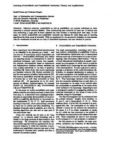
where U, L and P are the set of fuzzy variables, directed links between fuzzy variables, and conditional probability tables associated with directed links. Fig.1 illustrates the structure of a fuzzy causal probabilistic network where some nodes may receive crisp valued evidence which is mapped through a fuzzi er using membership functions to a vector of soft evidence, and some other nodes may generate crisp valued output through a defuzzi er. Except for the fuzzi ers and defuzzi ers, the rest of the structure is just a normal discrete Bayesian network. Note we do not delve into the inference algorithms. It suces to say that the existing inference algorithms for CPNs are naturally applicable for FCPNs. Fuzzi er While the dierence between fuzzy variables and crisp variables is the rst important signature of an FCPN from an ordinary CPN, however as a consequence, the most important characteristic of an FCPN is that in general, all the evidences are soft. For instance, hard evidence E(x ) for crisp variable x is a delta function as  x =x (14) E(x ) = 10 otherwise i

i

i

i

o i

which means x is found to be on the state x only. However, after mapping through the membership function  for the j-th fuzzy state X~ of the fuzzy variable u , for j = 1; 2; : : :; r , the fuzzy evidence for variable u turns out to be o i

i

ij

ij

i

i

i

E (ui ) = (i1 (xoi ) i2 (xoi ) : : : iri (xoi ))

(15)

Fig.2 (left) exempli es the fuzzi er which maps a crisp real variable x denoting temperature to a fuzzy variable u. The frame of x is the real interval X = [0; 45] in the unit of Celsius degree. The frame of u is the set of fuzzy states fcool; tepid; hotg. Each fuzzy state corresponds to a fuzzy set de ned through a fuzzy membership function  (x), u = cool; tepid; hot, on the same support set X. The fuzzy membership functions are shown in Fig.2. A crisp real temperature x = 27:5 as a crisp hard evidence is mapped through three membership functions to a vector of soft evidence u = (0 cool; 0:75 tepid; 0:25 hot). u

Fuzzy Variable

µ

X

Fuzzy Variable

U

µ

V

Y

Crisp Variable

Crisp Variable Fuzzifier

Defuzzifier

A Discrete Bayesian Network

A Fuzzy Bayesian Network

Figure 1. The general structure of a FCPN µ

µ

Fuzzy Membership Function Fuzzy Membership Function

µ cool

1.0

µ tepid

µ hot

1.0

µ tepid

0.625x

0.5

0.5 0.375x

0.0 0

x

o

5

o

10

o

15

o

20

o

25

o

30

o

35

x = 27.5 u=

o

40

o

45

o

o

C

0.0

Temperature

0

x o

5

0x

o

0 0.625 0.375

µhot

o

µ cool

10

o

15

o

20

o

25

o

30

u=

cool tepid hot

o

35

o

0 0.625 0.375

x = 27.5

40

o

45

o

o

C

Temperature

cool tepid hot

o

Figure 2. Fuzzi er (left) and Defuzzi er (right) Defuzzi er After the inference, the belief B(u ) for a fuzzy variable u is available. Note that the belief B(u ) is a vector i

i

i

B (ui ) = P (ui jE

~ i1 ); B (X ~ i2 ); : : : ; B (X ~ ir )) ) = (B (X i

(16)

where E denotes the whole set of evidence imposed on the set of fuzzy variables U. Sometimes, it is required to determine the most probable state x of the crisp variable x corresponding to the fuzzy variable u . This is usually referred to defuzzi cation from u to x . For FCPNs, a fuzzy node u is assigned a vector of probabilities after the inference as shown in (16), and each state X~ , j = 1; 2; : : :; r , is a fuzzy set. But all the states of u are de ned on the same crisp set X indexed by crisp variable x . We now need to determine the most probable crisp state x . The method proposed by Pan and McMichael (1998)[2] for defuzzi cation in a FCPN consists of two steps: o i

i

i

i

i

i

ij

i

i

o i

i

i

1. Uni cation. A unique fuzzy set X~ can be determined, which uni es all the fuzzy states X  ~ (x) =  (x)B(X~ ) i

ri

Xi

j

=1

ij

ij

2. Localization. A unique crisp point x can then be localized by using centroid method R x ~ (x)dx x = R  (x)dx ~

(17)

o i

o i

Xi

Xi

Xi

(18)

Xi

Fig.2 (right) shows how a defuzzi er works. For example, the belief on the node V which represents another temperature variable is (0 cool; 0:75 tepid; 0:25 hot). Now a crisp real temperature is to be determined from these fuzzy states. The rst step is to unify three membership functions with a weighted sum as expressed by (17). The area under the solid polyline is the uni ed fuzzy set. The second step is to calculate the centroid of the uni ed fuzzy set, which is e.g. x = 27:5.

3. MULTISENSOR DATA FUSION

Multisensor data fusion is a faculty inherent in any large information processing system which has to operate or survive in an unknown or dynamically changing physical environment with a high degree of autonomy or consciousness. Such a system would almost certainly be equipped with multiple sensors, taking many signi cant advantages of using multiple data sources over single ones. This faculty is inherent in biological systems and necessary in engineering systems. Animals and humans have evolved the capability to use multiple senses and to perform multisensory data fusion naturally to achieve more accurate assessment of the surrounding environment and identi cation of threats, thereby improving their chances of survival. Largely driven by military applications in the rst instances, data fusion technology has rapidly advanced in recent years from a loose collection of related techniques to an emerging true engineering discipline [12{15]. Applications of data fusion technology are widespread, and may be distinguished between military and nonmilitary ones. Non-military applications include robotics [16], remote sensing [17], monitoring and control of large engineering environments and systems, medical diagnosis, etc. Major military applications [18] include: building recognized air, sea or land pictures, airborne early warning, intelligence analysis, perimeter security, local area defence, counter-measure resistant systems, weapons guidance, target recognition and classi cation, battle eld surveillance, command and control. Sponsored by US Department of Defence, the Joint Directors of Laboratories (JDL) Data Fusion Working Group was established in 1986. One of their eorts was to codify the terminology related to data fusion. A data fusion process model created by JDL is illustrated in Fig.3 (adapted from [13]). More details of this model is explained in the next section. A much re ned model, called Analyst's Detection Support System (ADSS) [19], has been proposed by N.J. Redding from Australian Defence Science and Technology Organisation (DSTO) for target detection and threat estimation using multiple sensors and multiple sources of available information. The ADSS model is illustrated in Fig.4. This model is still under re nement and investigation. Whatever the application may be, the process of multisensor data fusion generally involves multiple data types such as sensor signals, features from the signal, physical and nominal attributes of physical objects, facts, decisions, knowledge, etc. Uncertainty including randomness and fuzziness exists everywhere in the process. Dierent data forms corresponding to dierent or even disparate information sources should be modelled by dierent to disparate fuzzy random variables. In line with these considerations, FCPNs provide a powerful modeling tool and computational architecture for multisensor data fusion and multisource information fusion in general. The next section describes a case study [20] on airborne early warning and control (AEW&C) as a defence application of multisensor data fusion using FCPNs.

DATA FUSION DOMAIN

Level One

Source Pre-Processing

Level Two

Object Recognition

Level Three

Situation Assessment

Threat Assessment Human Computer Interaction

Data Sources Database Management System

Support Databases

Fusion Databases

Level Four Process Refinement

Figure 3. Defence data fusion model used by US JDL.

Analyst

Analyst

Presentation

Information Fusion

Ordering

Threat

Ranking &

Estimation

Queueing

Information Fusion

Context

Detection

Behaviour

Military Geogr.

History

Models

Information

Vegetation & Terrain

Information Fusion

Prescreening

Change

Registration

Curvilinear

Tracks

Multilook &

Moving Target

Background

Backscatter

Modes

Models

Tracking

Features

Complex Models

Target Models

Features

Figure 4. Analyst's Detection Support System (ADSS) proposed by N.J. Redding, DSTO

4. A FCPN FOR AIRBORNE EARLY WARNING AND CONTROL (AEW&C)

The primary mission of an AEW&C mission system is that of surveillance and control. It requires the mission system to detect, classify, and track distant air targets, and to direct the simultaneous interception of multiple threat forces. However, the AEW&C system also performs other tasks, such as the coordination of search and rescue and airborne rendezvous control (e.g., airborne-tanker join-ups). In order to carry out these functions the mission system is equipped with a suite of sensors (radar, IFF, ESM, etc) (IFF = Identi cation, Friend or Foe, ESM = Electronic Support Measures), communication links, and sucient processing and database capacity to cope with large numbers of targets of dierent types under rapidly changing situation and threat levels [21]. Using on-board resources, the mission system must process and fuse data from multiple sensors and links in order to provide the commanders with relevant and timely information for controlling military operations. Speed and

accuracy in data and information processing are therefore paramount in all the component operations that make up the system. Clearly, unassisted manual operations can no longer meet the needs of such a system. Most of the data and information processing operations needed to transform sensor and link data into information useful for AEW&C operations therefore need to be fully automated. The various operations that contribute towards achieving the AEW&C objectives can be categorised under the four levels of the data fusion scheme (see Fig. 3) developed by the US Joint Directors of Laboratories Data Fusion Subpanel [22,12]. Level-1 operations involve the extraction of location and identity estimates from sensor and link data. Situation assessment is a level-2 operation and is the process by which the distributions of xed and moving entities generated by Level 1 are associated with environmental, doctrinal, and performance data (e.g., hostile vehicle tracability performance, sensor line-of-sight performance, etc). The task of situation assessment therefore involves identifying the probable situation causing the observed events and activities and typically requires a signi cant amount of a priori database information to support the component analyses. In general terms, the task involves categorising hypotheses according to some probability or con dence scale [12(pp. 277)]. Threat assessment is a level-3 operation and is the process by which the AEW&C quanti es the intent, destructive power as well as the vulnerability of the hostile force. Thus, whereas situation assessment establishes a view of activities, events, maneuvers, locations, and organisational aspects of force elements and from it estimates what is happening or going to happen, threat assessment estimates the degree of severity with which engagement events will occur [12(pp. 284)]. Sensor management and process control is a level-4 operation. It uses situation and threat assessment data to work out the deployment of sensors and other resources. The variety of threat scenarios requires that the AEW&C platform now be capable not only of detecting and reporting the threats, but also of tracking multiple threats and directing the engagement of those threats. The modern surveillance platform could therefore be categorised as a command and control platform as the direction of friendly tactical platforms (such as ghters and bombers) is an equally important part of the overall mission requirement. In such a platform the data and information processing is automated to a level that allows the majority of the AEW&C controller's time to be consumed with command and control functions rather than surveillance, situation, or threat assessment. Clearly, at this level of automation the AEW&C system is not simply a collection of sensors, links, databases, and processors. Instead, data and information from these sources are blended to continually present the most complete and accurate situational and threat assessment possible for the force commander. In the remainder of this section we present an approach to on-board sensor integration and how the resulting estimates can be used as evidence in a threat assessment algorithm that employs Bayesian networks as a basis for inference. The resulting Bayesian network could then be used to construct the corresponding FCPN.

4.1. The Generalised Tracker

In traditional tracking, kinematic measurements are processed to give estimates of target kinematic states (location, velocity, etc), while in traditional identi cation, nonkinematic measurements (frequency, radar PRF, cross-section area, IFF squitter, etc) are processed to give nonkinematic identity states. AEW&C missions are required to track and identify objects based on measurements that may have kinematic and nonkinematic parts. There is therefore a very strong need to unify tracking and identi cation in an optimal way. In general, tracking and identi cation are really complementary parts of the same activity, and if they are tackled together, there are savings in computation, increases in performance, and improvements in assessment of uncertainty. The generalised tracker, shown in Figure 5, is a level-1 algorithm that uni es tracking and identi cation and uses the augmented measurement-to-track association. It processes cluttered multisensor measurements from multiple targets and for each entity within the surveillance region, outputs an estimate of the uni ed state vector and its measure of uncertainty. It gives better track and identity estimates compared to algorithms in which tracking and identi cation are carried out separately and is compatible with a level-2 process that employs Bayesian networks as a basis for inference.

4.2. Situation and Threat Assessment for AEW&C

While situation and threat assessment for AEW&C systems can be implemented using several methods, Bayesian networks are preferred over other methods (e.g., experts systems, neural networks, Demster-Shafer, templating, etc) because they employ consistent reasoning and have representations of uncertainty that are consistent with the more

RADAR

IFF

Radar Signal Processor

IFF Signal Processor

ESM

ESM

Signal Processor

Data Association

Track Processing

Identity Estimation (IFF)

Identity Estimation (ESM)

+

Generalised Tracker

Generalised State Estimates for Level 2 Processes

Figure 5. Architecture of the generalised tracker. eective tracking algorithms. They employ rules that are soft and are expressed as conditional probabilities. Within each network, parent nodes can be updated using measurement entered at child nodes and child node probabilities can be updated using parent node probabilities. Node probability updates can be asynchronous. Hence, when a new report is received, the probability at the appropriate input node is adjusted, and this in turn is used to adjust all other probabilities within the network. Furthermore, the Bayesian network can be expanded to match the size and complexity of an application problem by increasing the number of nodes and causal links.

The Threat Assessment Model

As an illustration consider an air surveillance problem in which Bayesian network is used to derive target type probabilities and target intent probabilities given that the possible target types are restricted to: (1) ghter aircraft 1, (2) ghter aircraft 2, (3) helicopter, (4) missile, (5) commercial jetliner, (6) light civilian aircraft, and that the intent of a target is restricted to: (1) friendly, (2) neutral, and (3) hostile. Assume that the level-1 updates are from a generalised tracker that processes measurements from the primary surveillance radar, secondary surveillance radar (IFF), and ESM sensor. Fig. 6 is a Bayesian network that could be used to implement this target type and target intent estimation problem. The sensor reports from IFF, ESM, and radar are fused by the generalised tracker and the resulting uni ed object state vectors and measures of uncertainty are processed and used to update the dierent nodes within the Bayesian network. Such a system therefore consumes soft decisions from level-1 position and identity processes as well as information from data bases (e.g., ight corridors, aircraft dependent kinematics, environmental conditions, doctrines, etc), and outputs assessment of target type and intent. The applicable rules, written as conditional probabilities, can be described as follows: (1) The conditional probability p( AIRCRAFT DYNAMICS j AIRCRAFT TYPE ), depends on the velocity and acceleration constraints of the aircraft types, and the estimates, and the errors in the estimates, of the targets velocity and acceleration. (2) The conditional probability p( ESM j AIRCRAFT TYPE ), depends on the capability of dierent aircraft to produce a speci c ESM signature.

The Bayes Network ALLEGIANCE={FRIENDLY, NEUTRAL, HOSTILE} ALLEGIANCE

AIRCRAFT TYPE

TYPE={LIGHT CIVILIAN MISSILE FIGHTER HELICOPTER

IFF

COMMERCIAL JETLINER}

LOCATION

IFF={FRIENDLY NEUTRAL UNKNOWN}

DYNAMICS

ESM

COLLATERAL INFORMATION

Generalised Tracker

Radar

ESM

IFF

Figure 6. The Bayesian network model used for threat assessment. (3) The conditional probability p( OTHER j AIRCRAFT TYPE ), may use other information such as the characteristic Doppler signature of helicopters to determine the type of aircraft. (4) The conditional probability p( AIRCRAFT TYPE j INTENT ), takes into account the fact that hostile forces will use speci c aircraft in an assault. (5) The conditional probability p( IFF j INTENT ), is based on the fact that most friendly or neutral aircraft will be identi ed as such by an IFF sensor. (6) The conditional probability p( LOCATION j INTENT ), uses location information derived from the radar tracking to determine the probability that the aircraft is in a restricted military zone, or traversing a civilian air corridor. These six rules should allow correct probabilities to be assigned to aircraft types, and aircraft intent. Note that the links in the graph (and the conditional probabilities) actually refer to a set of rules, rather than one speci c IF THEN rule. In the remainder of this section we discuss Rule 1 and Rule 6 and how the conditional probabilities used to implement them are derived from estimates from the generalised tracker. Rule (1): p( DYNAMICS j AIRCRAFT TYPE ) One of the constraints of a particular aircraft is its velocity; for instance, a helicopter may hover (with zero speed), but its maximum speed will be lower than that of a ghter aircraft. The constraints placed upon the velocities of aircraft may be used to determine which type of aircraft is being tracked. To use the velocity constraints we require rules of the form p( V j AIRCRAFT TYPE ) where V = fE[x]; _ E[_y];  _ _ g are the means and covariances of velocity estimates. Inporder to perform inferences based on the aircraft velocity, the distribution of the velocity of the aircraft v = x_ 2 + y_2 must be derived from the generalised tracker estimates, and the probability of the aircraft's velocity falling within a particular set of constraints, given the velocity measurements, should be calculated. x;y

Rule (6): p( LOCATION j INTENT )

Civilian aircraft are restricted to speci c regions of the air, referred to here as corridors. In some cases these restrictions are carefully enforced especially near critical installations, while in other regions restrictions may be less rigid. Information about the restrictions on aircraft may be included in threat assessment by setting the conditional probability p( LOCATION j INTENT ) which gives the probability that an aircraft will appear in a particular location given its intent. In general only military aircraft (either friendly or unfriendly) will appear in restricted areas, though civilian aircraft may also appear in these areas accidentally. Thus the probabilities p( RESTRICTED LOCATION j INTENT = hostile) = high; (19) p( RESTRICTED LOCATION j INTENT = friendly) = high; (20) p( RESTRICTED LOCATION j INTENT = neutral) = low; (21) p( UNRESTRICTED LOCATION j INTENT = hostile) = moderate; (22) p( UNRESTRICTED LOCATION j INTENT = friendly) = moderate; (23) p( UNRESTRICTED LOCATION j INTENT = neutral) = high; (24) where the exact value of high, moderate and low in each case should be determined by local air restriction, and the degree to which they are enforced. In order to implement Rule 6 it is necessary to determine the probability that a target, whose position measurement includes errors, is in a speci c air corridor. Such probabilities can be deduced from the target's position and covariance estimates derived from the generalised tracker. An outline of the procedure is presented in the proceeding paragraph. The solution assumes a corridor de ned by two parallel lines given by the two equations a x = b, where a = (a0; a1) and b = (b0; b1). Assuming, without loss of generality, that b1 > b0, the solution is     (25) P fLocation is inside the corridorg = G bp1 ? a  ? G bp0 ? a  ; a a a a where  and  are the mean and covariance of the position estimates. The probability that a target is outside the corridor is simply one minus this probability. For more details of this work on AEW&C, see [20]. T

T

T

T

REFERENCES

T

1. H. Pan and D. McMichael, \Information fusion, causal probabilistic networks and Probanet I: Information fusion infrastructure and probabilistic knowledge representation," Proc. 1st International Workshop on Image Analysis and Information Fusion (IAIF'97) , pp. 445{458, 6-8 November 1997, Adelaide, Australia. 2. H. Pan and D. McMichael, \Fuzzy causal probabilistic networks - a new ideal and practical inference engine," Proc. 1st International Conference on Multisource-Multisensor Information Fusion , 6-8 July 1998, Las Vegas, USA. 3. H. Pan, D. McMichael, and M. Lendjel, \Inference algorithms in Bayesian networks and Probanet system," Digital Signal Processing - A Review Journal , to appear in 1998. 4. W. Buntine, \A guide to the literature on learning probabilistic networks from data," http://www.ultimode.COM/ wray/graphbib.ps.Z, 1998. 5. D. Heckerman, \Tutorial on learning in Bayesian networks," ftp://ftp.research.microsoft.com/pub/techreports/winter94-95/tr-95-06.ps. 6. P. Krause, \Learning probabilistic networks," http://www.auai.org/bayesUS krause.ps.gz, 1998. 7. F. Jensen, An Introduction to Bayesian Networks, UCL Press, 1996. 8. J. Pearl, Probabilistic Reasoning in Intelligent Systems: Networks of Plausible Inference, Morgan Kaufmann, San Mateo, CA, 1988. 9. S. Lauritzen and D. Spiegelhalter, \Local computations with probabilities on graphical structures and their applications to expert systems," Journal of Royal Statistical Society 50(2), pp. 157{224, 1988.

10. F. Jensen, S. Lauritzen, and K. Olesen, \Bayesian updating in causal probabilistic networks by local computations," Computational Statistics Quarterly 4, pp. 269{292, 1990. 11. D. McMichael, \Estimating the structure of Bayesian networks using mixtures," Proc. 1st International Conference on Multisource-Multisensor Information Fusion , 6-8 July 1997, Las Vegas, USA. 12. E. Waltz and J. Llinas, Multisensor Data Fusion, Artech House, Boston, 1990. 13. D. Hall and J. Llinas, \An introduction to multisensor data fusion," Proceedings of the IEEE Vol. 85, No. 1, pp. 6{23, January 1997. 14. N. Nandhakumar and J. Aggarwal, \Physics-based integration of multiple sensing modalities for scene interpretation," Proceedings of the IEEE Vol. 85, No. 1, pp. 147{163, January 1997. 15. M. L. II, I.Kadar, M. Alford, V.Vannicola, and S. Thomopoulos, \Distributed fusion architectures and algorithms for target tracking," Proceedings of the IEEE Vol. 85, No. 1, pp. 95{107, January 1997. 16. M. Kam, X. Zhu, and P. Kalata, \Sensor fusion for mobile robot navigation," Proceedings of the IEEE Vol. 85, No. 1, pp. 108{119, January 1997. 17. M. Daniel and A. Willsky, \A multiresolution methodology for signal-level fusion and data assimilation with applications in remote sensing," Proceedings of the IEEE Vol. 85, No. 1, pp. 164{180, January 1997. 18. D. McMichael, S. Halgamuge, G. Hamlyn, M. Karan, and N. Okello, Multisensor Data Fusion (Course Notes), Cooperative Research Centre for Sensor Signal and Information Processing, Adelaide, Australia, 1996. 19. N. Redding, \Analyst's Detection Support System," In: JP129 Ground Station Concepts for Broad-area Surveillance (U), Authors: Imaging Surveillance Systems, Australian Defence Science and Technology Organisation Report DSTO-CR-0089, 1998. 20. N. Okello, M. Roughan, and D. McMichael, Threat Assessment using Generalised Tracking and Bayes Nets, Re-

port No. 1/97, Cooperative Research Centre for Sensor Signal and Information Processing, Adelaide, Australia, 1997. 21. M. Long, Airborne Early Warning System Concepts, Artech House, 1992. 22. D. Hall, Mathematical Techniques in Multisensor Data Fusion, Artech House, 1992.