Generation of Random Bayesian Networks with Constraints on ...

Generation of Random Bayesian Networks with Constraints on Induced Width, with Application to the Average Analysis of d-Connectivity, Quasi-random Sampling, and Loopy Propagation Jaime S. Ide Fabio G. Cozman F´abio T. Ramos Escola Polit´ecnica, Universidade de S˜ao Paulo Departamento de Engenharia Mecatronica, Decision Making Lab Av. Prof. Mello Moraes, 2231 - CEP 05508900, S˜ao Paulo, SP - Brazil [email protected], [email protected], [email protected]

Abstract. We present algorithms for the generation of uniformly distributed Bayesian networks with constraints on induced width. The algorithms use ergodic Markov chains to generate samples, building upon previous algorithms by the authors. The introduction of constraints on induced width leads to more realistic results but requires new techniques. We discuss three applications of randomly generated networks: we study the average number of nodes d-connected to a query, the effectiveness of quasi-random samples in approximate inference, and the convergence of loopy propagation for non-extreme distributions.

1. INTRODUCTION Certain questions involving Bayesian networks are quite difficult to answer exactly. For example, what is the average number of variables that are d-connected to each other in a Bayesian network? Or, how do quasi-random importance sampling and quasi-random Gibbs sampling compare? Significant insight into such theoretical and empirical questions could be obtained analyzing large samples of Bayesian networks. However it does not seem likely that hundreds of “real” Bayesian networks will be freely distributed in the near future. We are left with an obvious solution: we must be able to randomly generate Bayesian networks for our experiments and comparisons. Many researchers have used ad hoc random processes to generate networks in the past (for example, [19, 22]); however we would like to produce networks that are uniformly distributed in some suitable space. The most challenging aspect of Bayesian network generation is exactly to define this space; that is, to define the properties that characterize “realistic” Bayesian networks. Our first attempt in generating Bayesian networks was to control the maximum node degree and the maximum number of edges, aiming to generate relatively sparse graphs [7]. We found that such a strategy is reasonable but not perfect. Restrictions solely on node degree and number of edges lead to “overly random” edges — real networks often have their variables distributed in groups, with few edges between groups.1 We then considered a number of other distingushing properties of “real” networks. For example, one option, suggested by T. Kocka, would be to produce graphs with a large number of equivalent graphs (a property observed in real networks). However we wanted to use properties with clear intuitive meaning — so that users of our algorithms would quickly grasp the properties of generated networks. We eventually found that the most appropriate quantity to control is the induced width of networks.2 The induced width of a network can be easily explained and understood; it conveys the algorithmic complexity of inferences and, indirectly, it captures how dense the network is. Our tests indicate (rather subjectively) that a network with low induced width “looks like” real networks in the literature. Besides, it makes sense to control induced width, as we are usually interested in comparing algorithms or parameterizing results with respect to the complexity of the underlying network, and induced width is the main indicator of such complexity. Unfortunately, the generation of random graphs with constraints on induced width is significantly more involved than the generation of graphs with constraints on node degree and number of 1 Tomas 2 Carlos

Kocka brought this fact to our attention. Brito suggested the idea.

B

F

B

F

D L

L

L

H

D

D

H

B

D L

H (a)

F

H (b) (c)

B

(d)

F

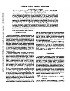
Figure 1: a) Network, b) moral graph, c) induced graph for ordering F, L, D, H, B, and d) induced graph for ordering L, H, D, B, F . Dashed lines represent induced connections.

edges. In this paper we report on new algorithms that accomplish generation of graphs with simultaneous constraints on all these quantities: induced width, node degree, and number of edges. Following our previous work [7], we divide the generation of random Bayesian networks into two steps. First we generate a random directed acyclic graph that satisfies constraints on induced width, node degree, and number of edges; then we generate probability distributions for the graph. To generate the random graph, we construct ergodic Markov chains with appropriate stationary distributions, so that successive sampling from the chains leads to the generation of properly distributed networks. The necessary theory is presented in Section 2.. Our algorithms are described in Section 3.. A freely distributed program for Bayesian network generation is presented in Section 4.. To illustrate how random Bayesian networks can be used, we describe three applications of obvious practical significance in Section 5.. First, we study the the average number of d-connected nodes in Bayesian networks. Second, we analyze the performance of quasi-random samples (as opposed to pseudo-random samples) in two inference algorithms: importance sampling and Gibbs sampling. Third, we investigate the convergence of loopy propagation on networks that have non-extreme distributions (that is, most probability values are far from zero and one).

2. BASIC CONCEPTS This section summarizes material from [7] and [5]. A directed graph is composed of a set of nodes and a set of edges. An edge (u, v) goes from a node u (the parent) to a node v (the child). A path is a sequence of nodes such that each pair of consecutive nodes is adjacent. A path is a cycle if it contains more than two nodes and the first and last nodes are the same. A cycle is directed if we can reach the same nodes while following arcs that are in the same direction. A directed graph is acyclic (a DAG) if it contains no directed cycles. A graph is connected if there exists a path between every pair of nodes. A graph is singly-connected, also called a polytree, if there exists exactly one path between every pair of nodes; otherwise, the graph is multiply-connected (or multi-connected for short). An extreme sub-graph of a polytree is a sub-graph that is connected to the remainder of the polytree by a single path. In an undirected graph, the direction of the edges is ignored. An ordered graph is a pair containing an undirected graph and an ordering of nodes. The width of a node in an ordered graph is the number of its neighbors that precede it in the ordering. The width of an ordering is the maximum width over all nodes. The induced width of an ordered graph is the width of the ordered graph obtained as follows: nodes are processed from last to first; when node X is processed, all its preceding nodes are connected (call these connections induced connections and the resulting graph induced graph). An example is presented at Figure 1. The induced width of a graph is the minimal induced width over any ordering; the computation of induced width is an NP-hard problem [5], and computations are usually based on heuristics [9]. A Bayesian network represents a joint probability density over a set of variables X [8]. The density is specified through a directed acyclic graph; every node in the graph is associated with a variable Xi in X, and with a conditional probability density p(Xi |pa(Xi )), where pa(Xi ) denotes the parents Q of Xi in the graph. A Bayesian network represents a unique joint probability density [15]: p(X) = i p(Xi |pa(Xi )) (consequence of a Markov condition). The moral graph of a Bayesian network is obtained by connecting

parents of any variable and ignoring direction of edges. The induced width of a Bayesian network is the induced width of its moral graph. An inference is a computation of a posterior probability density for a query variable given observed variables; the complexity of inferences is directly related to the induced width of the underlying Bayesian network [5]. We use Markov chains to generate random graphs, following [12]. Consider a Markov chain {Xt , t ≥ 0} over finite domains S and P = (pij )M ij=1 to be a M x M matrix representing transition probabilities, where M is the number of states and pij = P r(Xt+1 = j|Xt = i), for all t [16, 18]. The (s) s-step transition probabilities is given by P s = pij = P r(Xt+s = j|Xt = i), independent of t. A (s)

Markov chain is irreducible if for all i,j there exists s that satisfies pij > 0. A Markov chain is irreducible if and only if all pair of states intercommunicate. A Markov chain is positive recurrent if every state i ∈ S can be returned to in a finite number of steps; it follows a that finite irreducible chain is positive (s) recurrent. A Markov chain is aperiodic if the greatest common divisor of all those s for which pii > 0, (s) is equal to one (that is, G.C.D.(s|pii > 0) = 1). Aperiodicity is ensured if pii > 0 (pii is a self-loop probability). A Markov chain is ergodic if there exists a vector π (the stationary distribution) satisfying (s) lims−→∞ pij = πj , for all i and j; a finite aperiodic, irreducible and positive recurrent chain is ergodic. A PN transition matrix is called doubly stochastic if the rows and columns sum to one (that is, if j=1 pij = 1 PN and i=1 pij = 1). A Markov chain with such a transition matrix has a uniform stationary distribution [16].

3. GENERATING RANDOM DAGS In this section we show how to generate random DAGs with constraints on induced width, node degree and number of edges. After such a random DAG is generated, it is easy to construct a complete Bayesian network by randomly generating associated probability distributions — if all variables in the Bayesian network are categorical, probability distributions are produced by sampling Dirichlet distributions (for details see [7]). To generate random DAGs with specific constraints, we construct an ergodic Markov chain with uniform limiting distribution, such that every state of the chain is a DAG satisfying the constraints. By running the chain for many iterations, eventually we obtain a satisfactory DAG. Algorithm PMMixed produces an ergodic Markov chain with the required properties (Figure 2). The algorithm is significantly more complex than the algorithms presented in [7]. The added complexity comes from the constraints in induced width — however such a price is worth paying as the resulting DAGs are much more “realistic” representatives of Bayesian networks. The algorithm works as follows. We create a set of n nodes (from 0 to n − 1) and a simple network to start. The loop between lines 03 and 08 constructs the next state (next DAG) from the current state. Lines 05 and 08 verify whether the induced width of the current DAG satisfies the maximum value allowed; constraints on maximum node degree and maximum number of edges must also be checked there. If the current DAG is a polytree, the next DAG is constructed in lines 04 and 05; if the current DAG is multi-connected, the next DAG is constructed in lines 07 and 08. Depending on the current graph, different operations are performed (the procedures AorR and AR correspond to the valid operations). Note that the particular procedure to be performed and the acceptance (or not) of the resulting DAG is probabilistic, parameterized by p. Algorithm PMMixed is essentially a mixture of procedures AorR and AR. The first procedure is used in [7] to produce multi-connected graphs with constraints on node degree; the second procedure is used in [7] to produce polytrees with constraints on node degree. We need both to guarantee irreducibility of Markov chains when constraints on induced width are present; the procedure AR creates a needed “path” in the space of polytrees that is used in Theorem 3. The mixture of procedures has two other benefits: first, it creates more complex transitions, hopefully increasing the convergence of the chain; second, it eliminates a restriction on node degree that was needed in [7]. The PMMixed algorithm can be understood as a sequence of probabilistic transitions that follow the scheme in Figure 3.

Algorithm PMMixed: Generating DAGs with induced width control Input: Number of nodes (n), number of iterations (N ), maximum induced width, and possibly constraints on node degree and number of nodes. Output: A connected DAG with n nodes. 01. Create a network with n nodes, where all nodes have just one parent, except the first node that does not have any parent; 02. Repeat N times: 03. If current graph is a polytree: 04. With probability p, call Procedure AorR; with probability (1 − p), call Procedure AR. 05. If the resulting graph satisfies imposed constraints, accept the graph; otherwise, keep previous graph; 06. else (graph is multi-connected): 07. Call Procedure AorR. 08. If the resulting graph is a polytree and satisfies imposed constraints, accept with probability p; else accept if it satisfies imposed constraints; otherwise keep previous graph. 09. Return current graph after N iterations.

Procedure AR: Add and Remove 01. Generate uniformly a pair of distinct nodes i, j; 02. If the arc (i, j) exists in the current graph, keep the same state; else 03. Invert the arc with probability 1/2 to (j, i), and then 04. Find the predecessor node k in the path between i and j, remove the arc between k and j, and add an arc (i, j) or arc (j, i) depending on the result of line 03.

Procedure AorR: Add or Remove 01. Generate uniformly a pair of distinct nodes i, j; 02. If the arc (i, j) exists in the current graph, delete the arc, provided that the underlying graph remains connected; else 03. Add the arc if the underlying graph remains acyclic, otherwise keep same state. Figure 2: Algorithm for generating DAGs, mixing operations AR and AorR.

p

AorR

multiconnected

polytree 1-p

polytree

AR

p

accept

polytree

If polytree 1-p multiconnected

AorR

reject

If multiconnected

Figure 3: Structure of PMMixed.

multiconnected

i

j

k

i

(a)

j

k (b)

1

n

2 (c)

Figure 4: Simple trees used in our proofs: (a) Simple tree, (b) Simple polytree, (c) Simple sorted tree.

We now establish ergodicity of Algorithm PMMixed. Theorem 1 The Markov chain generated by Algorithm PMMixed is aperiodic. Proof. It is always possible to stay in the same state for procedures AR and AorR; therefore, all states have a self-loop probability greater than zero. QED Theorem 2 The transition matrix defined by the Algorithm PMMixed is doubly stochastic. Proof. If we have symmetric transition probabilities between two neighbor states, its rows and columns sum one, because the self-loop probabilities are complementary to all other probabilities. Procedure AorR is clearly symmetric; procedure AR operation is also symmetric [7]. We just have to check that transitions between polytrees and multi-connected graphs are symmetric; this is true because transitions from polytree to multi-connected are accepted with probability p, and multi-connected to polytree transitions are also accepted with the same probability. QED We need the following lemma to prove Theorem 3. Lemma 1 After removal of an arc from a multi-connected DAG, its induced width does not increase. Proof. When we remove an arc, the moral graph stays the same or contains less arcs; by just keeping the same ordering, the induced width cannot increase. QED Theorem 3 The Markov chain generated by Algorithm PMMixed is irreducible. Proof. Suppose that we have a multi-connected DAG with n nodes; if we prove that from this graph we can reach a simple sorted tree (Figure 4 (c)), the opposite transformation is also true, because of the symmetry of our transition matrix — and therefore we could reach any state from any other (during these transitions, graphs must remain acyclic, connected and must satisfy imposed constraints). So, we start by finding a loop cutset and removing enough arcs to obtain a polytree from the multi-connected DAG [15]. The induced width does not increase during removal operations by Lemma 1. From a polytree we can move to a simple polytree (Figure 4 (b)) in a recursive way. For all extreme sub-graphs of our polytree, for each pair of extreme sub-graphs (call them branches), it is possible to “cut” a branch and add it in the other branch, by the procedure AR, without ever increasing the induced width. Doing this we get a unique branch. If we have more than two branches connected to a node, we repeat this process by pairs; we do this recursively until get a simple polytree. Now that we have a simple polytree, we get a simple tree (Figure 4 (a)) just inverting arcs to the same direction, without ever getting an induced width greater than two. The last step is to get a simple sorted tree (Figure 4 (c)) from the simple tree. The idea here is illustrated in Figure 5. We want to sort labelled nodes from 1 to n. Start removing arc (n, k) and adding arc (l, i) (step 1 to 2). Remove arc (j, n) and add arc (n − 1, n) (step 2 and 3). Note that in this configuration, the induced width is one. Now, remove arc (n − 1, o) and add arc (j, k) (step 3 and 4). Repeat steps 2 and 4 for all nodes. So, from any multi-connected DAG it is possible to reach a simple sorted tree. The opposite path is clearly analogous, so we can go from any DAG to any other DAG, and the chain is irreducible. Note that constraints on node degree and maximum number of edges can be dealt with within the same processes. QED By the previous theorems we obtain: Theorem 4 The Markov chain generated by Algorithm PMMixed is ergodic and its unique stationary converges to a uniform distribution. The algorithm PMMixed can be implemented quite efficiently, except for the computation of induced width — finding this value is a NP-hard problem with no easy solution. There are heuristics for computing induced width; some of which have been found to be of high quality [9]. Consequently, we must change our goal: instead of adopting constraints on exact induced width, we assume that the user specifies

step 1

i

j

n

step 2

k

l

i

k

l

j

n

n step 3

k

n-1

step 4

o

j

o

k

j

n-1

n

Figure 5: Basic moves to obtain a simple sorted tree.

Procedure J: Sequence of AorR 01. If the current graph is polytree, repeat with probability (1 − p − q): 02. Generate uniformly a pair of distinct nodes i, j; 03. If arc (i, j) does not exist in current graph, add the arc; otherwise, keep the same state. 04. If the current graph is multi-connected, repeat with probability (1 − p − q): 05. Generate uniformly a pair of distinct nodes i, j. 06. If arc (i, j) exists in current graph, remove the arc; otherwise, keep the same state. 07. If the new graph satisfies imposed constraints, accept the graph; otherwise, keep previous graph. Figure 6: Procedure J.

a maximum width given a particular heuristic. We call this width the heuristic width. Our goal then is to produce random DAGs on the space of DAGs that have constraints on heuristic width. Apparently we could still use the PMMixed algorithm here, with the obvious change that lines 05 and 08 must check heuristic width instead of induced width. However such a simple modification is not sufficient: because heuristic width is usually computed with local operations, we cannot predict the effect of adding and removing edges on it. That is, we cannot adapt Lemma 1 to heuristic width in general, and then we cannot predict whether a “path” between DAGs can in fact be followed by the chain without violating heuristic width constraints. We must create a mechanism that would allow the chain to transit between arbitrary DAGs regardless of the adopted heuristic. Our solution is to add a new type of operation, specified by procedure J (Figure 6) — this procedure allows “jumps” from arbitrary multi-connected DAGs to polytrees. We also assume that any adopted heuristic is such that, if the DAG is a polytree, then the heuristic width is equal to the induced width. Even if a given heuristic does not satisfy this property, the heuristic can be easily modified to do so: test whether the DAG is a polytree and, if so, return the induced width of the polytree (the maximum number of parents amongst all nodes). Procedure J must be called with probability (1 − p − q) both after line 04 and after line 07 in the algorithm PMMixed. The complete algorithm can be understood as a sequence of probabilistic transitions that follow the scheme in Figure 7. All previous theorems can be easily extended to this new situation; the only one that must be substantially modified is Theorem 3. Transitions from polytree to multi-connected DAGs are performed with probability (1 − q); transitions from multi-connected DAGs to polytrees are q = 1 − q. The value of p and q control the mixing rate of the performed with probability 1 − (p + q) × p+q chain; we have observed remarkable insensitivity to these values.

p

AorR

multiconnected

polytree q

polytree

AR

1-p-q Jump

multiconnected

If p/(p+q)

accept

polytree

polytree q/(p+q)

p+q

reject AorR

multiconnected

If multiconnected

multiconnected

1-p-q Jump

polytree

Figure 7: Structure of PMMixed with procedure J.

4. BNGENERATOR The algorithm PMMixed (with the modifications indicated in Figure 7) can be efficiently implemented with existing ordering heuristics, and the resulting DAGs are quite similar to existing Bayesian networks. We have implemented the algorithm using a O(n log n) implementation of the minimum weight heuristic. The result is the BNGenerator package, freely distributed under the GNU license (at http://www.pmr.poli.usp.br/ ltd/Software/BNGenerator).3 An example network generated by BNGenerator is depicted in Figure 8. The BNGenerator accepts specification of number of nodes, maximum node degree, maximum number of edges, and maximum heuristic width (for minimum weight heuristic, but other heuristics can be added). The software also performs uniformity tests using a χ2 test. Such tests can be performed only for relatively small number of nodes (as the number of possible DAGs grows extremely quickly [17]), but they allowed us to test the algorithm and its procedures. We have observed the relatively fast mixing of the chain with the transitions we have designed.

5. APPLICATIONS To show how to use our previous results, we have selected three problems that have received some analysis in the literature but have no conclusive solution yet. Due to the lack of space, we present a brief summary of rather extensive tests. 5.1. D-CONNECTIVITY Given a node Xq and a set of nodes XE , the number of nodes d-connected to Xq given XE is a fundamental quantity in Bayesian networks. This quantity indicates how many variables are “requisite” for an inference; it is also indicates how large a sensitivity analysis must be [2]; it essentially controls the complexity of the EM algorithm when learning networks [23]; and it can be used to eliminate redundant computations in learning [3]. Despite the importance of d-connectivity, there seems to be no result in the literature indicating the relationship between heuristic width (the “complexity” of the network) and the expected number of dconnected nodes. We illustrate how such a relationship could be investigated with random networks. We took an ensemble of random networks with medium number of nodes and heuristic width, as these networks are the ones most often used (currently at least) in exact inference and in learning. For each 3 The software uses the facilities in the JavaBayes system, including the efficient implementation of ordering heuristics (http://www.cs.cmu.edu/˜javabayes).

Figure 8: Bayesian network generated with BNGenerator and opened with JavaBayes: 30 nodes, maximum degree 20, maximum induced width 2.

Table 1: Average number of d-connected nodes given number of nodes (N ) and heuristic width (HW ).

(N, HW ) ↓ 35,4 35,8 70,4 70,8

3% 13 ± 6 17 ± 7 23 ± 9 34 ± 11

14% 19 ± 5 23 ± 5 36 ± 10 49 ± 7

28% 21 ± 7 27 ± 4 39 ± 16 55 ± 7

85% 13 ± 9 20 ± 9 13 ± 12 31 ± 17

network, we computed the number of d-connected nodes for a random queried variable, varying the number of observed nodes. We considered situations where 3%, 14%, 28% and 85% of the nodes are observed. The first two situations correspond to typical queries in Bayesian networks, where the last situation corresponds to a typical inference in an EM algorithm [3]. The situation of 28% observed nodes is an intermediate case. Table 1 presents results for four different sets of networks, for different sizes and heuristic width (each entry summarizes 5000 networks). Note the interesting fact that the number of d-connected nodes is larger for the “intermediate” case, decreasing in other cases. Note also the relatively large number of d-connected nodes: for an heuristic width of 4, about 35% of the nodes are d-connected even when a small number of variables are observed. 5.2. QUASI-RANDOM INFERENCES In this section we look into the behavior of Monte Carlo methods associated with quasi-random numbers; that is, numbers that form low discrepancy sequences — numbers that progressively cover the space in the “most uniform” manner [14]. There have been quite successful applications of quasi-Monte Carlo methods for integration in low-dimensional problems; in high-dimensional problems, there has been conflicting evidence regarding the performance of quasi-Monte Carlo methods. As a positive example, Cheng and Druzdzel obtained good results in Bayesian network inference with importance sampling using quasirandom numbers [1]. There has been little work combining quasi-random numbers to Gibbs sampling; finding efficient methods is still an open problem [6]. The difficulty seems to be the deleterious interaction between correlations in quasi-random sequences and Markov chains. Liao applied quasi-random numbers for variance reduction in a Gibbs sampler for classical statistical models [10], obtaining good but not conclusive results through randomly permuted quasi-random sequences. We have investigated the following question: How does quasi-random numbers affect standard

Table 2: Average Mean Square Error (multiplied by 103 ) for importance sampling (top) and Gibbs sampling (bottom).

Imp. Samp. Pseudo Quasi

0 1.2 ± 0.07 1.9 ± 0.4

10 5.5 ± 2.8 7.3 ± 3.3

20 19.0 ± 2.6 17.3 ± 13.3

Gibbs Samp. Pseudo Quasi

0 3.4 ± 0.5 79.3 ± 8.2

10 3.4 ± 0.6 81.6 ± 10

20 3.2 ± 0.8 82.6 ± 13

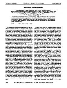
importance sampling and Gibbs sampling algorithms in Bayesian networks? We have used the importance sampling scheme derived by Dagum and Luby [4], and have investigated networks with Halton sequences as quasi-random numbers. The summary of our investigation is as follows. First, pseudo-random numbers are clearly better than quasi-random numbers in medium-sized networks for Gibbs sampling. Second, pseudo-random number have a small edge over quasi-random numbers for importance sampling; however the differences are so small that both can be used. In fact it is not hard to find networks that behave better under quasi-random importance sampling than under pseudo-random importance sampling.4 It should also be noted that both importance sampling and Gibbs sampling are affected in different ways by observations, as predicted by the theory [4]. As we increase the number of observations, importance sampling eventually turns into a much worse option than Gibbs sampling (corroborating results by Cheng and Druzdzel, as their importance sampling algorithm displays a notable degradation in performance when observations are added [1, Figures 7 and 8]). These conclusions are illustrated by Table 2, where we show the Mean Square Error (as defined in [1]) for sets of networks under various algorithms. All networks had 100 nodes and heuristic width 5. Each row shows the MSE for different numbers of observed nodes (0, 10 and 20 nodes). 5.3. LOOPY PROPAGATION Loopy propagation algorithms are based on the iterative application of Pearl’s propagation algorithm in multi-connected graphs [11]. These algorithms have been observed to often converge quickly to correct answers. In fact, little is known about convergence, except for a few special cases [21, 20]. Existing analysis of loopy propagation have identified a few situations where the algorithm does not converge, but has not found a definite explanation for lack of convergence [13]. One of the essential aspects of the “nonconvergent” networks in [13] was the presence of logical nodes, with zero/one probability values. So, we pose the question: how does loopy propagation behave when probabilities are not extreme, as we perform inference in large and dense networks? We have never observed, in a rather comprehensive exploration, situations where loopy propagation failed to converge when probabilities are larger than zero. We have varied the number of nodes (going up to 500 nodes), maximum heuristic width (up to 28), number of values for variables, and even tried to introduce somewhat extreme distributions into our networks; we never forced loopy propagation to oscillate. Even for large networks where no known exact algorithm could succeed, loopy propagation converged. In most cases convergence led to correct (or approximately correct) values; however, the quality of approximations is not always excellent — and it seems that the longer the algorithm takes to converge, the worst the result. To illustrate an interesting experiment with random networks, in Figure 9 we show the relationship between heuristic width and number of iterations to convergence for a fixed family of networks. The number of nodes is 100, and all variables are binary. We took rather complex networks, in the sense that heuristic width was quite high (up to 28). The absolute error is just the absolute value of the difference between the correct inference and the inference generated by loopy propagation. Note that the absolute error and the number of interactions to convergence are almost independent of heuristic width. We would have expected 4 As a notable (not randomly generated) example of this phenomenon, the Alarm network does behave slightly better with quasirandom importance sampling than with pseudo-random importance sampling (corroborating results by Cheng and Druzdzel [1]).

Absolute Error

Loopy Propagation Errors

0.04 0.02 0 10

12

14

16

18

20

22

24

26

28

Heuristic Width

Interations

Loopy Propagation Convergence 20 10 0 10

12

14

16

18

20

22

24

26

28

Heuristic Width Figure 9: Absoluter error, number of iterations, and induced width (test with 200 random networks; bars indicate variance within 10 random networks).

that the more dense the network, the more difficult it would be for loopy propagation to converge — but loopy propagation seems to be incredibly robust in this respect. The absolute error is considerably large in many of these tests.

6. CONCLUSION In this paper we have presented what we believe is the best available solution for the generation of random Bayesian networks. The key idea is to generate DAGs with constraints on induced width, and then generate distributions associated with the generated DAG. Given the NP-hardness of induced width, we have resorted to “heuristic width” — the width produced by one of the many high-quality heuristics available. We generate DAGs using Markov chains, and the need to guarantee heuristic width constraints leads to a reasonably complex transition scheme encoded by algorithm PMMixed and procedure J. The algorithm can be easily changed to accommodate a number of other constraints (say constraints on the maximum number of parents). We have observed that this strategy does produce “realistic” Bayesian networks. We have presented three applications of these random networks. First, we have investigated the relationship between induced width and d-connectivity, verifying that the number of d-connected nodes tends to be rather large in realistic networks. Such a quantity impacts inference algorithms, sensitivity analysis, and learning algorithms such as EM. Second, we have confirmed comments in the literature that suggest that standard Gibbs sampling cannot profit from quasi-random samples, while straightforward importance sampling presents essentially the same behavior under pseudo- and quasi-random sampling for medium-sized networks. Third, we have shown that loopy propagation converges with extraordinary regularity and robustness when nonextreme distributions are used, and that the convergence of the algorithm does not seem to be affected by the complexity of the underlying networks.

Acknowledgements We thank Carlos Brito for suggesting us use the induced width, Robert Castelo for pointing us to Melanc¸on et al’s work, Guy Melanc¸on for confirming some initial thoughts, Nir Friedman for indicating how to generate distributions, and Haipeng Guo for testing the BNGenerator. We also thank Jaap Suermondt, Alessandra Potrich and Tomas Kocka for providing important ideas, and Y. Xiang, P. Smets, D. Dash, M. Horsh, E. Santos, and B. D’Ambrosio for suggesting valuable procedures.

The first author was supported by FAPESP grant 00/11067-9. The third author was supported by HP Labs and was responsible for investigating loopy propagation; we thank Marsha Duro from HP Labs for establishing the funding and Edson Nery from HP Brazil for managing it. The work received substantial and generous support from HP Labs. The work was also partially supported by CNPq through grant 300183/98-4.

References [1] Jian Cheng and J. Druzdzel, Marek. Computational investigation of low-discrepancy sequences in simulation algorithms for bayesian networks. In Craig Boutilier and Moises Goldszmidt, editors, Proceedings of the 16th Conference on Uncertainty in Artificial Intelligence (UAI-00), pages 72–81, SF, CA, June 30– July 3 2000. Morgan Kaufmann Publishers. [2] Veerle Marleen H. Coup´e, Linda L. C. van der Gaag, and J. D. F. Habbema. Sensitivity analysis: an aid for belief-network quantification. Knowledge Engineering Review, 15:1–18, 2000. [3] Fabio Gagliardi Cozman. Removing redundancy in the expectation-maximization algorithm for Bayesian network learning. In Leliane Nunes de Barros, Roberto Marcondes, Fabio Gagliardi Cozman, and Anna Helena Reali Costa, editors, Workshop on Probabilistic Reasoning in Artificial Intelligence, pages 21–26, S˜ao Paulo, 2000. Editora Tec Art. [4] Paul Dagum and Michael Luby. An optimal approximation algorithm for Bayesian inference. Artificial Intelligence, 93(1–2):1–27, 1997. [5] Rina Dechter. Bucket elimination: An unifying framework for probabilistic inference. In Eric Horvitz and Finn Jensen, editors, Proceedings of the 12th Conference on Uncertainty in Artificial Intelligence (UAI-96), pages 211–219, San Francisco, August 1–4 1996. Morgan Kaufmann Publishers. [6] K. T. Fang and Y. Wang. Number Theoretic Methods in Statistics. Chapman & Hall, New York, 1994. [7] J. S. Ide and F. G. Cozman. Random generation of bayesian networks. In Proc. of XVI Brazilian Symposium on Artificial Intelligence. Springer-Verlag, 2002. [8] F. V. Jensen. An Introduction to Bayesian Networks. Springer-Verlag, New York, 1996. [9] U. Kjaerulff. Triangulation of graphs — algorithms giving small total state space. Technical Report R-9009, Department of Mathematics and Computer Science, Aalborg University, Denmark, March 1990. [10] J. G. Liao. Variance reduction in Gibbs sampler using quasi random numbers. Journal of Computational and Graphical Statistics, 7(3):253–266, September 1998. [11] R. J. McEliece, D. J. C. MacKay, and J. F. Cheng. Turbo decoding as an instance of Pearl’s ’belief propagation’ algorithm. IEEE Journal on Selected Areas in Communication, 16(2)(CSD-99-1046):140–152, 1998. [12] G. Melanon and M. Bousque-Melou. Random generation of dags for graph drawing. Technical Report technical report INS-R0005, Dutch Research Center for Mathematical and Computer Science-CWI, 2000. [13] K. P. Murphy, Y. Weiss, and M. I. Jordan. Loopy belief propagation for approximate inference: An empirical study. In In Proceedings of the Fifteenth Conference on Uncertainty in Artificial Intelligence, pages 467–475, 1999. [14] Harald Niederreiter. Random Number Generation and Quasi-Monte Carlo Methods, volume 63 of CBMSNSF regional conference series in Appl. Math. SIAM, Philadelphia, 1992. [15] J. Pearl. Probabilistic Reasoning in Intelligent Systems. Morgan-Kaufman, 1988. [16] Sidney I. Resnick. Adventures in Stochastic Processes. Birkh¨auser, Cambridge, MA, USA; Berlin, Germany; Basel, Switzerland, 1992. [17] R. W. Robinson. Counting labeled acyclic digraphs. In F. Harary, editor, New Directions in the Theory of Graphs, pages 28–43, Michigan, 1973. Academic Press.

[18] S. M. Ross. Stochastic Processes. John Wiley and Sons; New York, NY, 1983. [19] Peter Spirtes, Clark Glymour, and Richard Scheines. Causation, Prediction, and Search (second edition). MIT Press, 2000. [20] Sekhar C. Tatikonda and Michael I. Jordan. Loopy belief propagation and Gibbs measures. In Adnan Darwiche and Nir Friedman, editors, Conference on Uncertainty in Artificial Intelligence, pages 493– 500, San Francisco, California, 2002. Morgan Kaufmann. [21] Yair Weiss and William T. Freeman. Correctness of belief propagation in Gaussian graphical models of arbitrary topology. Technical Report CSD-99-1046, CS Department, UC Berkeley, 1999. [22] Y. Xiang and T. Miller. A well-behaved algorithms for simulating dependence structure of bayesian networks. In International Journal of Applied Mathematics, volume 1, pages 923–932, 1999. [23] Nevin Lianwen Zhang. Irrelevance and parameter learning in Bayesian networks. Artificial Intelligence, 88:359–373, 1996.